
The Ultimate Trading Strategy: How to Combine Kelly Criteria and Monte Carlo Simulation

A Gambling Problem
Have you ever stared down at your hand in a game of Texas Hold’em, knew your hand was good enough to bet, but didn’t know how much to throw in the middle? Or have you ever had a fairly good trading strategy, but you weren’t sure how much money to yolo into the markets? You’re not the only one. Bet sizing, whether it’s in poker, sports, or the stock market is just as important as the strategy you're using to determine when to play. What do we do in this situation? Do we throw everything in and pray you’re running hot at the table? Or do we take a more conservative route and always bet 10% of your stack. Ideally, we would bet whatever generates the most wealth in the long term, but flawed thinking often gets in the way. Too many times, I have seen a poker tournament lost or a trade turn bad because of something idiotic. It might be as simple as thinking the dealer is out to get you, so you play a little more conservative, or that the hot girl that blew on the dice was really good luck, so you stuck everything in there. We know logically neither of these are good long-term strategies, but people blow billions in Vegas and in the market. If only there was a simpler solution for bet sizing. I introduce The Kelly Criterion!
The OG
In John Kelly’s original paper, he derived a formula used for bet sizing in gambling. The formula depended on three factors:
- p: the probability of a win,
- q = 1-p: the probability of a loss
- b: the odds or payout (ratio you stand to win over the amount you stand to lose).
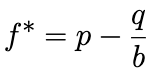
f* represents the percentage of our total stack we should be putting at risk.
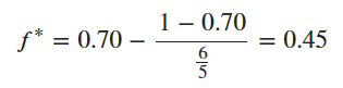
Let's try an example…. What percent would the Kelly formula tell us to bet if we have a 70% chance with 6:5 odds? You have 5 seconds to figure it out. 5.4.3.2.1. 45%! So, if we have $100 bankroll the Kelly Criteria is telling us we should be betting $45 from our stack.
There are some changes we have to make to apply this to a stock market, but this can be used where you lose 100% of the capital if you lose the bet. So, things like blackjack and sports betting can use this formula. To see how this formula compares to a continuous betting strategy see below…
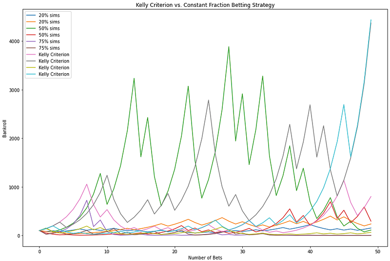
The picture above has 2 simulations of betting at 20%, 50%, and 75% and 4 at the Kelly Criterion amount. There is a 60% chance of a winning a coin flip. This graph is important because it shows while the Kelly Criterion may give you the optimal allocation to generate the greatest amount of wealth in the long run, it does not mean it will always be successful. It is not a predictive tool and should be combined with other risk management strategies. Check out our YouTube channel if you’d like to see a short tutorial on how this was made.
The Proof is in the Pudding
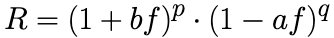
Before we get into the Kelly Criterion for the markets, I want to make sure we all have a firm footing on how and why the Kelly Criterion works. The Kelly Criterion works by maximizing the expected value of the logarithm of wealth. From our studies in Calculus 2 we know we can find the maximum of a curve by finding the derivative of a continuous function. To start we need to find out a formula that measures our wealth. First, we should remember that since we are trying to maximize wealth, we are going to need a growth rate that is based on compounding bets. Keeping with our notation above we will use p to represent the probability of a win, q for the probability of a loss (1-p), b as the payout, and f for the portion of money we want to wager. For ease of use we are also going to use R for rate of growth and a for amount you lose if you lose the bet.
Since this is compounding, we start with our growth rate as:
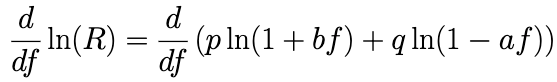
We want to find the derivative of this but as with anything with exponents and derivatives this will be easier if we apply some natural logs to both sides. Then we can take the derivative

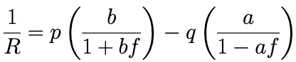
Now since we want this to equal 0, we can replace 1/R with 0 and solve for f.
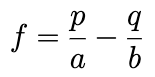
Now this might be slightly different than our original gambling Kelly Criterion equation but remember in our derivation we were assuming a is the percent we lose. Imagine a hand of blackjack, if you lose the hand then you lose 100% of the bet, so if we set a to 1 then we get back to our original Kelly formula.
Betting the Market
Now as you can probably guess from our derivation there is a way to use the Kelly formula in the stock market. Unlike some gambling games we can limit our downside in a trade. The most basic way to use the Kelly Criterion in the market is to take the same formula as above, but instead of making a 1, make it whatever value you’d be ok with losing. This will calculate the new % you should be betting.
There is a different way to go about using Kelly Criterion as described by Edward Thorpe in his paper The Kelly Criterion in Blackjack Sports Betting, and the Stock Market. Thorpe’s work on using the Criteria results in the equation below:
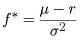
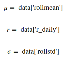
In this equation μ are the mean returns, r is the risk-free rate, and σ is the standard deviation of returns. A few important things to consider when using this Thorpe formula. We will still need accurate data to estimate the mean and standard deviation of a security. This will be determined by the look-back period. Unfortunately, there is no answer on how long the look-back period should be, that’ll be up to you to figure out. When trading securities like this you’ll also have to frequently rebalance the optimal Kelly value as your balance shifts, timing will be up to you again.
From Theory to Practice: Applying the Kelly Criteria and Monte Carlo Simulation to Trade the SPY
The caveats described above present a challenge in transitioning from understanding the Kelly Criteria in theory to actually being able to use it. It’s like when you learn how to drive well with an instructor. As soon you’re alone in the car, you put the pedal to the floor, have about 15 seconds of excitement, then crash into a ditch. Allow us to be your instructor that stays in the car…. for a while. In this section I’ll be showing you how to apply the Kelly Criteria to trade the SPY. We will see how the Kelly Criteria does by itself as well as in combination with some safety precautions.
We will apply Thorpe’s Kelly Criteria to trade the SPY in six different ways in order to visualize its strengths and weakness. In all six strategies we will be buying and holding the SPY. Each day, we will use the Kelly Criteria to allocate a percentage of our portfolio towards buying and holding the SPY (equity), the remaining percentage will be held as unused cash. Thus, the combination of our equity and cash for each day will give our total value of our portfolio.
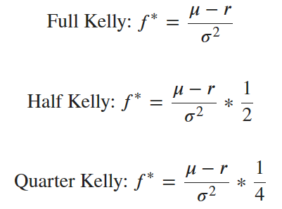
- Full Kelly [we allocate exactly how much the equation tells us to]
- Half Kelly [we allocate half of the specified percentage]
- Quarter Kelly [we allocate a quarter of the specified percentage]
- Monte Carlo Cap 3 Full Kelly [a Full Kelly, limited to a maximum leverage of 3.0 (300%), using z-score from Monte Carlo simulation as a scaled exit]
- Monte Carlo Cap 3 Half Kelly [a Half Kelly, limited to a maximum leverage of 3.0 (300%), using z-score from Monte Carlo simulation as a scaled exit]
- Monte Carlo Cap 3 Quarter Kelly [a Quarter Kelly, limited to a maximum leverage of 3.0 (300%), using z-score from Monte Carlo simulation as a scaled exit]
Now for the first three strategies: All three implement Thorpe’s Kelly in essentially the same way. The following equations show the explicit differences.
As I describe the process of backtesting these strategies, I will identify specific elements of the code (full code available at the bottom of this article). However, for a more detailed breakdown of the code, refer to the upcoming video on our YouTube channel.
First, we obtain the several years' worth of SPY price history and treasury rate history using the function: get_price_and_rate_history().
Next, we extract the information from our data that correspond to the variables of Thorpe’s Kelly Criteria using the function: Kelly(data, period, kelly_cap=None, kelly_frac=1). In this equation μ are the mean returns, r is the risk-free rate, and σ is the standard deviation of returns.
Now that we have all the required values, we are ready to run our backtest using the function: long_Kelly_strat(data, period)
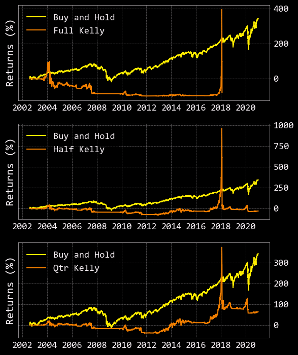
In the above output, Buy and Hold is what would happen if we bought 1 dollar worth of the SPY on our starting date in 2002 and held until late in 2020. As you can see, our % returns following Full, Half, and Quarter Kelly allocations result in a drop below zero at different points in time. This is akin to the new driver crashing into a ditch without a seatbelt situation I described above. Just like cars, the Kelly Criteria can be very useful, however, proper safety precautions must be taken to prevent you (AKA your account) from going kaput.
So, how can we prevent the Kelly Criteria from overleveraging our account and making us very susceptible to sharp downturns? One thing we can do is cap the maximum Kelly value at 3, thereby allowing us to leverage no more than 300% of our portfolio. Three hundred percent leveraged?! Sounds like a lot to me too. If only there was a way for us to predict the probability of the SPY continuing in the upward direction?! Such a prediction would allow us to take profit if the probability of the SPY continuing upward was low.
If you’ve been following our page, you’re probably thinking that we can predict future prices of the SPY by using a Monte Carlo Simulation, as we did in our previous post, Application of Ito Calculus: Monte Carlo Simulation, and its accompanying video on YouTube. We were also able to obtain the probability of any one outcome from the Monte Carlo results distribution.

Keep in mind, the stochastic differential equation (SDE) that we used in our previous article uses the same historical mu and sigma that the Kelly Criteria uses. We will stick with that SDE for familiarity’s sake. You could very likely improve the predictive ability of the Monte Carlo by using another SDE that is not limited to historic inputs, one such SDE would be the Merton-Jump Equation.
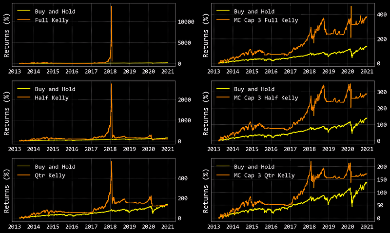
In order to use the MC in conjunction with the Kelly Criteria. We need to run a MC each day to estimate the probability distribution of the following day’s close price. At the close of the next day, we can look back at the likelihood that yesterday’s price reached today’s close. Now that we understand this relationship, we can use the z-score of today’s close price to determine how many standard deviations away it is from the mean of yesterday’s MC simulation. If the z-score is > 1, we can conclude that the chance of the SPY price continuing in an upward direction is less likely than moving in a downward direction. Therefore, if the z-score is > 1, we will set the Kelly Criteria to the side and begin to exit our position proportionally to the z-score minus 1. For example, if the z-score = 1.25, and z-score - 1 = 0.25, we would subsequently exit 25% of our current SPY position.
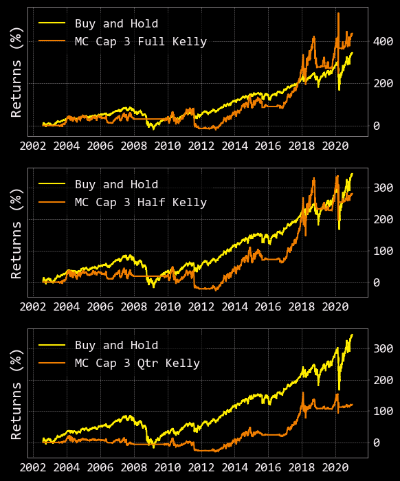
Below are the results of a backtest using Full, Half, and Quarter Kelly values (capped at 3.0) and Monte Carlo Simulations (for scaled exiting of our positions). In the long run, these results significantly outperform the backtests that did not incorporate the cap and Monte Carlo. However, if you look closely, all of the equity curves for our strategies fall below 0 at some point in their path… thus, we busted our accounts again :(
Don’t fret young grasshopper, all is not lost.
Beware the Single, Beautiful Backtest
If you read enough trading blogs/articles/posts, you will undoubtedly come across many authors claiming a strategy will dominate the market as evidenced by one pretty picture and a return of 700+%. I cannot say if their strategies are good or bad, but I will say that their backtests are likely overfit to the specific timeframe they are showing you.
Take the Kelly Monte Carlo strategies above for instance. The ‘MC Cap 3 Full Kelly’ outperformed the SPY by nearly 100% over the whole-time frame, which is a positive sign. Had we been trading this strategy in real life however, we would have never seen that performance because our account would have run down to nothing sometime in late 2011.
What about if we started trading these strategies in 2013? Well, our ‘MC Cap 3 Full Kelly’ strategy would have ABSOLUTELY MURDERED the SPY returns by over 200%!!!
My point is… the best way to know if a strategy will work in real life is not to test it over one long continuous timeframe, but rather to chunk up that long timeframe into smaller random samples. By testing the performance of your strategy on many smaller timeframes, you’ll be able to obtain more accurate statistics of its potential future performance.
Conclusion
Up to this point you should feel confident in your understanding of the function of the Kelly Criteria to approximate appropriate bet sizing in many scenarios. You should also be aware of the limitations of the Kelly Criteria in its tendency to increase your exposure to sudden changes in market dynamics. I hope that you also have a better understanding of what to look for when analyzing your own strategies and the strategies of others. With any idea that you think will be a winner in the market, your goal should always be to prove yourself wrong. If you approach ideas in this manner, may not feel fantastic in the short term as you find holes in your ideas, but you will feel fantastic in the long term when you have a flourishing portfolio instead of no portfolio. Finally, as I’ve demonstrated in this article, the combination of the Kelly Criteria and Monte Carlo Simulations can prove successful in certain timeframes and fail in others. In future articles, we will be building upon the potential of this strategy by incorporating other risk management techniques!
Check out our Link Tree to find our profiles on YouTube, Instagram, and TikTok and join us next time as we wander deeper into the market.
Please feel free to comment with any questions, concerns, or topics you would like covered in future posts!
If you found this or any of our other content valuable, please consider buying us a coffee.
**THIS CONTENT IS NOT FINANCIAL ADVICE. IT IS STRICTLY EDUCATIONAL**
Full Code
import warnings
warnings.filterwarnings('ignore')
import pandas as pd
import numpy as np
%matplotlib inline
import matplotlib.pyplot as plt
import yfinance as yf
from openbb_terminal.sdk import openbb
from tqdm import tqdm

# Interactive tables in Jupyter Notebook/Lab
from itables import init_notebook_mode
init_notebook_mode(all_interactive=True)

# Interactive tables in Google Colab
#from google.colab import data_table
#data_table.enable_dataframe_formatter()

def get_price_and_rate_history():

    bad_start = '2001-07-31'
    good_start = '2012-04-01'
    end = '2020-12-31'
    # price history
    data = yf.download('SPY', start=good_start, end=end)
    # we just need close data
    data.drop(['Open', 'High', 'Low', 'Volume', 'Adj Close'],
              axis=1,
              inplace=True)

    # obtain US Treasury nominal 1-month rate for risk free rate
    rates = openbb.economy.treasury(maturities=['1m'],
                                    frequency='daily',
                                    start_date=good_start,
                                    end_date=end)
    # remove the % from the rates
    rates /= 100
    # fill rates for all days by filling missing days with the last value
    # this makes sure no days of price data are lost when joining
    rates = rates.resample('D').last().ffill()
    data = data.join(rates)
    data.rename(columns = {'Nominal_1-month':'1m_rate'}, inplace = True)

    return data

def Kelly(data, period, kelly_cap=None,kelly_frac=1):

    data['returns'] = data['Close'].pct_change()
    data['log_returns'] = np.log(data['Close'])-np.log(data['Close'].shift(1))
    data['rollstd'] = data.log_returns.rolling(period).std()
    data['rollmean'] = data.log_returns.rolling(period).mean()
    data['r_daily'] = np.log((1+data['1m_rate']) ** (1/period))

    # kelly value = ((mu - r) / sigma**2) * kelly_frac
    data['kelly_value'] = ((data['rollmean']-data['r_daily'])
                            /data['rollstd']**2)*kelly_frac

    # convert to 0 all kelly_values that are <= 0
    data['kelly_factor'] = np.where(data.kelly_value < 0, 0, data.kelly_value)
    data['kelly_factor'] = np.where(data.kelly_factor >= kelly_cap,
                                    kelly_cap,
                                    data.kelly_factor)

    # put a max cap on the kelly factor
    if kelly_cap:
        data['kelly_factor'] = np.where(data.kelly_factor >= kelly_cap,
                                        kelly_cap,
                                        data.kelly_factor)
    data = data.dropna()

    return data

def monte_carlo_simulation(num_sims, sim_steps, X0, mu, sigma, T):
    '''
    num_sims (int): the number of simulations to run
    sim_steps (int): the number of steps in each simulation
    X0 (float): the initial value of the stock
    mu (float): expected return
    sigma (float): the volitility of the stock
    T (int): the time horizon of the simulation
    '''

    dt = T / sim_steps
    W = np.cumsum(np.random.randn(num_sims, sim_steps) * np.sqrt(dt), axis=1)
    X = X0 * np.exp((mu - 0.5 * sigma ** 2) * dt + sigma * W)

    # calculate the mean and std
    final_vals = X[:, -1]
    mean = round(np.mean(final_vals), 2)
    stdev = round(np.std(final_vals), 2)

    return pd.Series([mean, stdev])

def fill_monte(data, period):

    # monte carlo for each iteration of the data so daily
    mc_results = data.apply(lambda row: monte_carlo_simulation(num_sims=10000,
                                                               sim_steps=period,
                                                               X0=row['Close'],
                                                               mu=row['rollmean'],
                                                               sigma=row['rollstd'],
                                                               T=1), axis=1)

    mc_results.rename(columns = {0:'mc_mean', 1:'mc_std'}, inplace = True)

    # join mc_mean and mc_std tuples as data columns
    data = data.join(mc_results)
    # create a column of the upper price bound (1 standard deviation from the mean)
    data['up1'] = data.mc_mean + data.mc_std
    # shift the up1, mc_mean, and mc_std columns by 1 day -- allows us to assess
    # if we are outside the upper bound of the previous day's monte carlo
    data[['up1', 'mc_mean', 'mc_std']] = data[['up1', 'mc_mean', 'mc_std']].shift(1)

    return data

def long_Kelly_strat(data, period, MC=False):

    # generates np array for length of sim to track portfolio ratios
    cash = np.zeros(data.shape[0])
    equity = cash.copy()
    portfolio = cash.copy()

    # starts portfolio and cash at 1
    portfolio[0] = 1
    cash[0] = 1
    equity[0] = 0

    for i, _row in enumerate(tqdm(data.iterrows())):
        if i >= 1:
            # this assigns row to all the data in 1 period of the data so the index, close, returns, log returns, kelly_factor
            row = _row[1]
            # If there is no kelly value then the portfolio just adds the previous time period's portfolio and cash
            if np.isnan(row['kelly_factor']):
                portfolio[i] += portfolio[i-1]
                cash[i] += cash[i-1]
                continue

            if MC == True:

                z = (row['Close'] - row['mc_mean']) / row['mc_std']

                portfolio[i] += (cash[i-1] * (1 + row['r_daily'])) + (equity[i-1] * (1 + row['returns']))

                # if outside of 1 standard deviation, exit the percent of the position equal to z score minus 1
                if z > 1.0:
                    equity[i] = equity[i-1] * (1 + row['returns'])
                    cash[i] = cash[i-1] * (1 + row['r_daily'])

                    amt_out = equity[i] * (z-1)
                    equity[i] -= amt_out
                    cash[i] += amt_out

                # if z score within 1 standard deviation or less than, use kelly criteria to allocate position
                else:
                    #reweights portfolio for each iteration of the data so daily
                    equity[i] += portfolio[i] * row['kelly_factor']
                    cash[i] += portfolio[i] * (1- row['kelly_factor'])

            else:
                #reweights portfolio for each iteration of the data so daily
                portfolio[i] += (cash[i-1] * (1 + row['r_daily'])) + (equity[i-1] * (1 + row['returns']))
                equity[i] += portfolio[i] * row['kelly_factor']
                cash[i] += portfolio[i] * (1- row['kelly_factor'])

    data['cash'] = cash
    data['equity'] = equity
    data['portfolio'] = portfolio
    data['strat_returns'] = data['portfolio'].pct_change()
    data['strat_log_returns'] = np.log(data['portfolio']) - np.log(data['portfolio'].shift(1))
    data['strat_cum_returns'] = data['strat_log_returns'].cumsum()
    data['cum_returns'] = data['log_returns'].cumsum()

    return data

period = 252

k_data = get_price_and_rate_history()
mc_data = get_price_and_rate_history()

reg_k_data = Kelly(k_data, period, kelly_frac=1)
half_k_data = Kelly(k_data, period, kelly_frac=.5)
qtr_k_data = Kelly(k_data, period, kelly_frac=.25)

reg_mc_data = Kelly(mc_data, period, kelly_cap=3, kelly_frac=1)
half_mc_data = Kelly(mc_data, period, kelly_cap=3, kelly_frac=.5)
qtr_mc_data = Kelly(mc_data, period, kelly_cap=3, kelly_frac=.25)

reg_mc_data = fill_monte(reg_mc_data, period)
half_mc_data = fill_monte(half_mc_data, period)
qtr_mc_data = fill_monte(qtr_mc_data, period)

reg_kelly = long_Kelly_strat(reg_k_data, period)
half_kelly = long_Kelly_strat(half_k_data, period)
qtr_kelly = long_Kelly_strat(qtr_k_data, period)

mc_reg_kelly = long_Kelly_strat(reg_mc_data, period, MC=True)
mc_half_kelly = long_Kelly_strat(half_mc_data, period, MC=True)
mc_qtr_kelly = long_Kelly_strat(qtr_mc_data, period, MC=True)

# Plot Everything
fig, ax = plt.subplots(3, 2, figsize=(12, 8))

# Control
SPY = (np.exp(reg_kelly['cum_returns']) -1) *100

# Reg Kelly
reg_cumrets = (np.exp(reg_kelly['strat_cum_returns']) -1) *100
ax[0, 0].plot(SPY , label='Buy and Hold')
ax[0, 0].plot(reg_cumrets, label='Full Kelly')
ax[0, 0].set_ylabel('Returns (%)')
ax[0, 0].legend()

half_cumrets = (np.exp(half_kelly['strat_cum_returns']) -1) * 100
ax[1, 0].plot(SPY, label='Buy and Hold')
ax[1, 0].plot(half_cumrets, label='Half Kelly')
ax[1, 0].set_ylabel('Returns (%)')
ax[1, 0].legend()

qtr_cumrets = (np.exp(qtr_kelly['strat_cum_returns']) -1) * 100
ax[2, 0].plot(SPY, label='Buy and Hold')
ax[2, 0].plot(qtr_cumrets, label='Qtr Kelly')
ax[2, 0].set_ylabel('Returns (%)')
ax[2, 0].legend()

mc_reg_cumrets = (np.exp(mc_reg_kelly['strat_cum_returns']) -1) *100
ax[0, 1].plot(SPY, label='Buy and Hold')
ax[0, 1].plot(mc_reg_cumrets, label='MC Cap 3 Full Kelly')
ax[0, 1].set_ylabel('Returns (%)')
ax[0, 1].legend()

mc_half_cumrets = (np.exp(mc_half_kelly['strat_cum_returns']) -1) * 100
ax[1, 1].plot(SPY, label='Buy and Hold')
ax[1, 1].plot(mc_half_cumrets, label='MC Cap 3 Half Kelly')
ax[1, 1].set_ylabel('Returns (%)')
ax[1, 1].legend()

mc_qtr_cumrets = (np.exp(mc_qtr_kelly['strat_cum_returns']) -1) * 100
ax[2, 1].plot(SPY, label='Buy and Hold')
ax[2, 1].plot(mc_qtr_cumrets, label='MC Cap 3 Qtr Kelly')
ax[2, 1].set_ylabel('Returns (%)')
ax[2, 1].legend()

fig.tight_layout()
fig.subplots_adjust(top=0.88)
plt.show()


