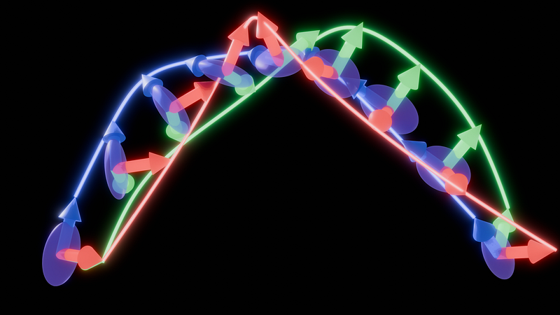
The Rigid Body Lagrangian and the Inertia Tensor

There’s more to the world than point particles.

This is stop 22 on The Road to Quantum Mechanics.

Up to this point in the series, we’ve covered models for the motion of particles, gravity, electromagnetism, waves, heat, and light. While we’ve certainly done a lot, we still have an omission so glaring that we couldn’t even model most objects in our world.

Most physical objects that you could touch kind of work like particles, but have some extent in space. While we could model these objects as collections of individual points (and we usually have to for soft-bodies), many objects are rigid — they don’t noticeably stretch or squish in any way. These objects are called rigid bodies. In this article, we’ll come up with a precise mathematical model for rigid bodies, derive the form of the Lagrangian, and set ourselves up to derive Euler’s Rigid Body Equations.

Check Your Understanding

We’re going to once again have some standard proofs, derivations, calculations, and Physical modeling. I’ve also put deriving Euler’s Rigid Body Equations from the facts in this article into the mix.

Proving that SO(n) Has n(n – 1)/2 Free Continuous Parameters

Prove that SO(n) has n(n – 1)/2 free continuous parameters. As a hint, note that

n(n – 1)/2 is the sum of the first n – 1 natural numbers,
a unit vector in n dimensions has n – 1 free continuous parameters,
and proof by induction exists.

Alternatively, you might be able to use the fact that is the number of ways to choose two things from n objects without replacement where order doesn’t matter.

Common Inertia Tensors

Calculate the inertia tensors for the following objects.

A sphere
A cylinder of uniform density
A cylinder of uniform density with a hole cut out of it like a rolled up piece of paper
A cone

Rolling Down a Hill

Assume an object is rolling straight down a hill without slipping. Use the Lagrangian approach to predict its motion. [Hint: The translational velocity and the rotational velocity are linearly related.]

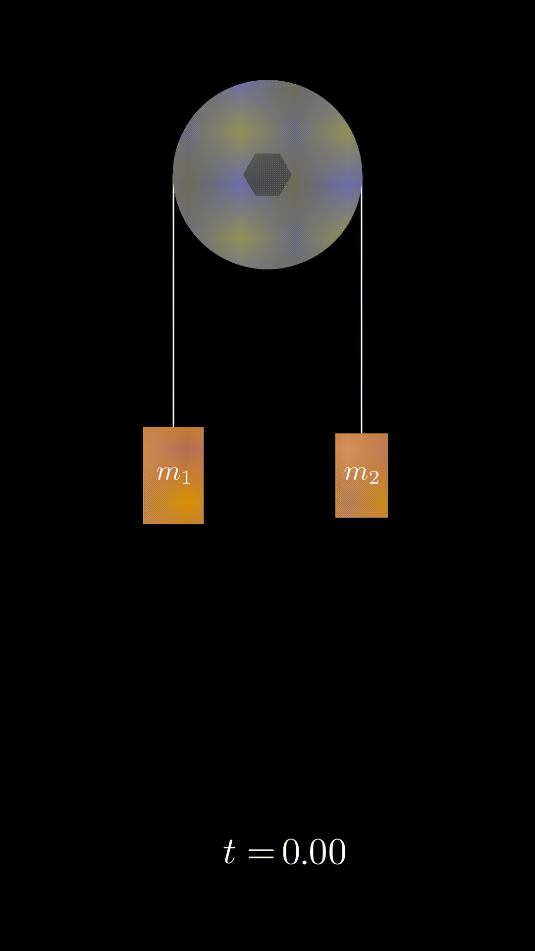
Pulleys

Figure out the equations of motion for the system below under the assumption that the pulley is a cylinder of uniform density.

Physical Pendulum

A physical pendulum is a rigid body that rotates around a fixed point, usually under the force of gravity. Use the Lagrangian approach to find the equations of motion. [Hint: You should get a result known as the Parallel-Axis Theorem.]

Euler’s Rigid Body Equations*

Use the Lagrangian at the end of this article and the Euler-Lagrange equations to derive Euler’s Rigid Body Equations. I don’t want to leave you too high and dry, so here are some hints.

The translational velocity does not show up Euler’s Rigid Body Equations.
The derivative of the potential with respect to the orientation θ should give you the torque.
The inertia tensor depends on time, and we can express that dependence with the angular velocity.

Prerequisites

You should read Lagrangian Mechanics, An Intro to Tensors, and whatever I’m currently calling this article.

Distance-Preserving Transformations of Space

So now, we just have to figure out every distance-preserving transformation of 3D Euclidean space and remove anything that doesn’t fit. But what is distance? And how do we measure it? If you’ve gotten this far in the series, it shouldn’t surprise you that we can define the distance between two points as the length of the vector between them.

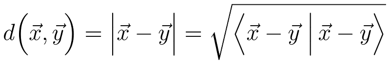
So now, a distance preserving transformation has to preserve the inner product for the difference between every pair of vectors u and v.

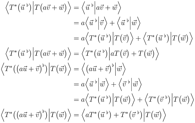
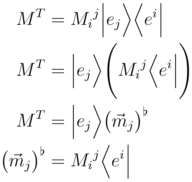
The Dual Transformation

There’s a slight issue with the notation above, though. If we define T : V ↦ V, where V is the vector space, then T cannot act on the dual vector space. To deal with this problem, I’m going to define T * : V * ↦ V * (the notation means the function T * maps a covector to another covector) such that

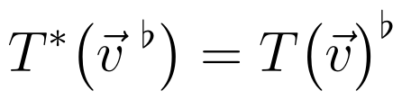
In other words, if T maps a vector u to v, then T * maps the covector u to v.

Translations

Note that u and v only show up in the form u – v. When we only care about the difference between two objects, we can always add the same constant to both objects. In this case, we can add the same vector to all points.

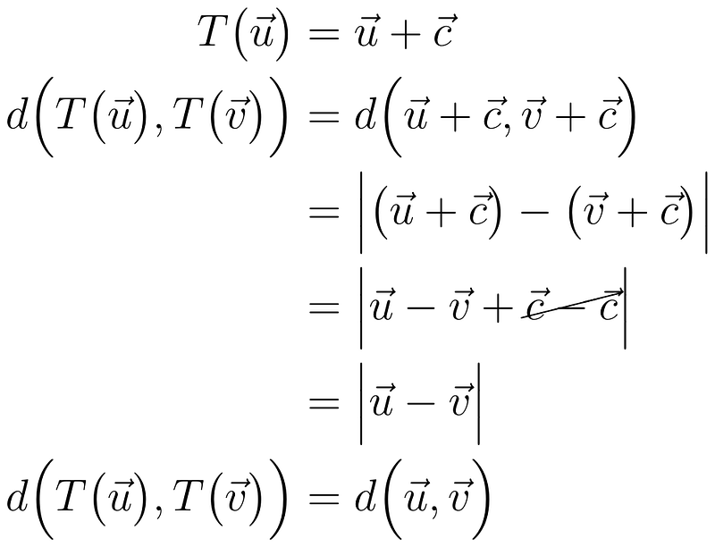
Such a transformation is known as a translation. Since we can only add vectors to other vectors, this is the only transformation of this form that we can allow.

Linearity

We can only use the fact that we’re taking the difference between two vectors in our distance formula to determine that translations preserve distance. Once we’ve established that, we can replace the difference of the two vectors with just an arbitrary vector. In other words, we’re looking for any transformation that preserves the lengths of vectors, which is equivalent to making sure the transformation preserves the inner product between vectors. Since the inner product is linear, the transformation must also be linear.

With this fact, we can explicitly write out the form of the transformation as the matrix

which means the dual transformation is the transpose (or the Hermitian conjugate if we were working with complex vectors), which we get by flipping the rows and the columns or the bras and kets.

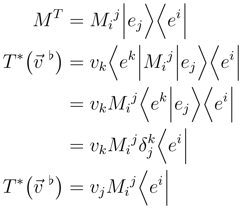
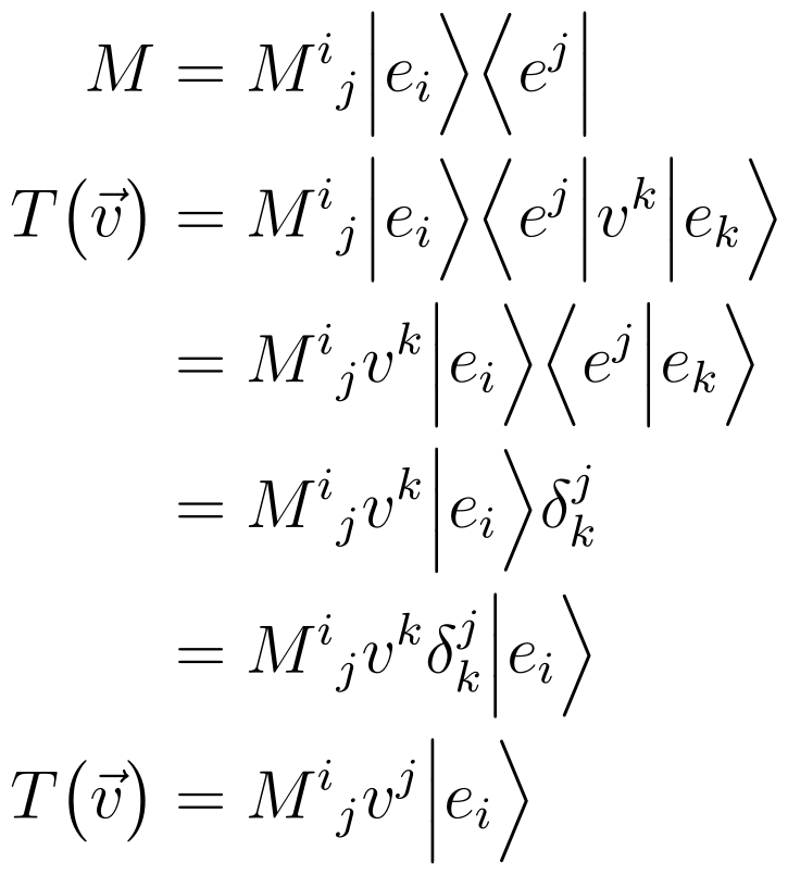
Matrix Representations

Now, we just need to write everything out.

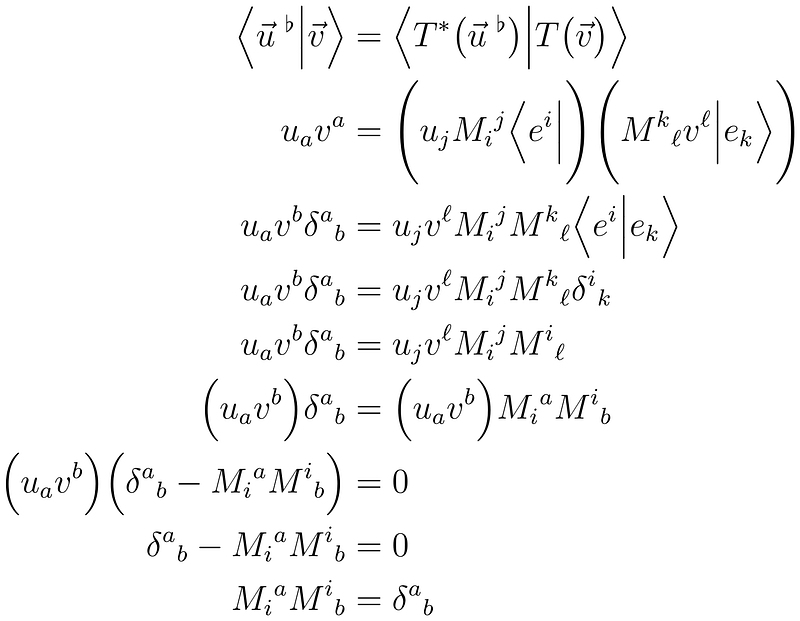
This last equation means that we need the product of the matrix with its transpose to be the identity matrix.

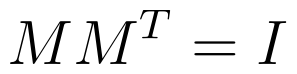
We now have to figure out what this matrix means.

Orthogonal Matrices

It’s often helpful to think of matrices as a change of basis where each column determines where you send one of the basis vectors. Why this interpretation works becomes clear in any representation if we just apply the matrix to the basis vectors.

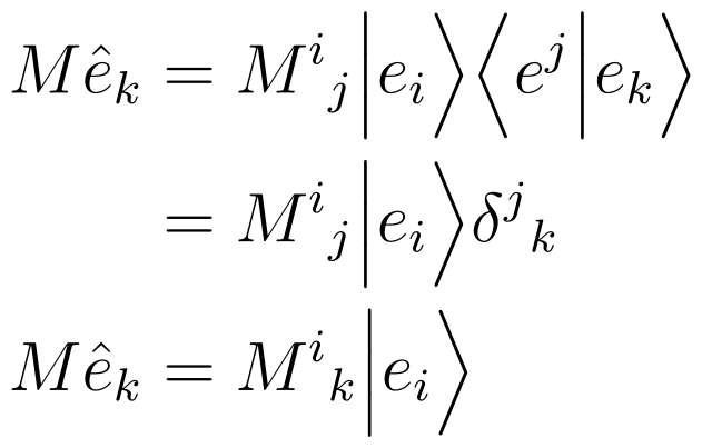
We can represent the columns of matrices by factoring out the ket part of each matrix and making it into a vector.

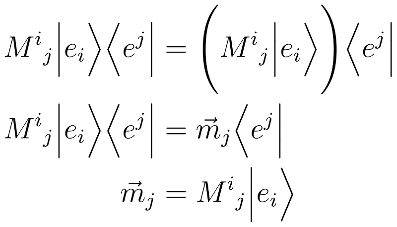
Likewise, we can find the corresponding covector by factoring out the bra part of the transposed matrix.

Now, if we apply one of these covectors to one of these vectors, we have

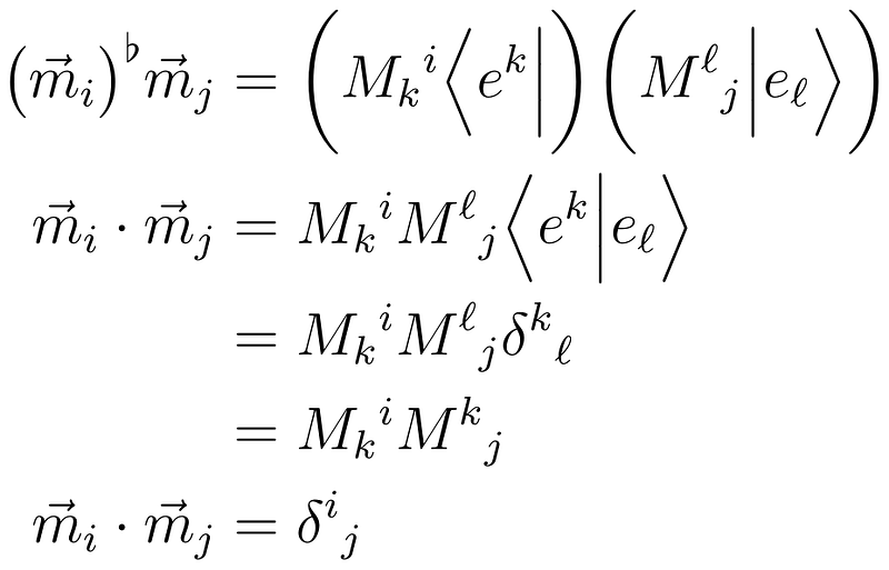
In other words, the columns of our matrix must be orthonormal, which is why we call these orthogonal matrices.

Orthogonal Transformations

So we’ve come up with some abstract description of these matrices, but what transformations do these matrices represent? Before we get into any kind of proof, we should try to look at some examples. To get these examples, I’m going to generate random numbers for each column that follow all the given constraints and look where the vectors are sent. For the first column, we have to have a unit vector. For the second column, we get that we have to have a unit vector that’s orthogonal to the first unit vector. This orthogonality reduces our dimension of possible choices by one, which gives us any unit vector in the plane normal to our first vector. For the last column, we get a unit vector that’s entirely orthogonal to both vectors. There are only two choices. If we put some examples together, we get

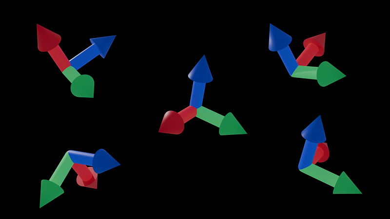
From this image, it should be clear that all of these transformations can be represented as some combination of rotations and flips.

Rigid Body Transformations

Since translations, rotations, and flips are the only distance-preserving transformation in Euclidean space, rigid body motion can only involve translations, rotations, and flips. While it’s possible to translate and rotate a rigid body, it is impossible to flip a rigid body. Such a transformation would require that all the points in the rigid body instantaneously teleport, which does not happen, so the rigid body transformations are translations and rotations.

Rigid Body Coordinates

We can describe translations in N dimensions with N free parameters: one for each coordinate of the vector. On the other hand, rotations are a bit trickier. We know that there are at most N² free parameters for any square matrix in N dimensions. Furthermore, every linear equation removes one of these free parameters. Since we want the vectors to be orthonormal, we get N(N – 1)/2 equations to make sure the vectors are orthogonal and N equations to make sure each vector is normalized. If we assume that all of these equations are linearly independent, then we have N² – [N(N – 1)/2 + N] = N(N – 1)/2 free parameters. The list below has the number of parameters for rigid body transformations in N dimensions.

1D: 0 parameters
2D: 1 parameter
3D: 3 parameters
4D: 6 parameters
…

As we can see, there are zero ways to rotate a 1D system because there’s no 1D continuous transformation that keeps every point somewhere on the line and keeps the distance between points the same. In 2D, we can only rotate clockwise or counterclockwise, and we can parameterize the rotation with a single real number. In 3D, we can use choose two numbers to pick the axis of rotation (say latitude and longitude) and one number to represent how much we’re rotating around the axis. We can’t really visualize things in 4D, so I’ll stop here.

Building Up SO(n) and O(n) Transformations From Lower Dimensions

Picking a unit vector gets rid of one of the possible dimensions, which means we can decompose an O(n) or SO(n) transformation into an O(n – 1) or SO(n – 1) transformation about a specific axis. For example, in 3D, we can pick an axis and then rotate around that axis with an SO(2) transformation.

A Preview of Lie Groups

We’ll talk in much more depth about Lie Groups later when we talk about Hamiltonian Mechanics, but I might as well mention them while we’re here.

(ℝⁿ, +): The Lie Group of all translations (It’s just the standard vector space.)
O(n): The Orthogonal Group in n dimensions. It contains all rotations and flips but no translations.
SO(n): The Special Orthogonal Group in n dimensions. It contains all rotations but no flips.
E(n) or ISO(n): The Euclidean Group. It contains all the distance-preserving transformations of translations, rotations, and flips.
SE(n): The Special Euclidean Group or Rigid Motions in n dimensions. It contains all the translations and rotations, but no flips.

We’re going to be using the Special Euclidean Group to work with rigid bodies.

Standard Representation of SO(n)

SO(n) is the easier to represent, since we can represent it as the product of matrices of the form

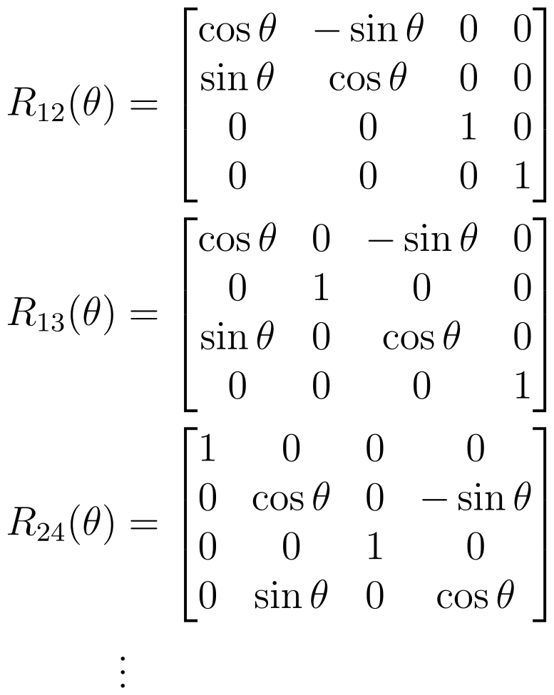
With this representation, the N(N – 1)/2 free continuous parameters show up as the angles of the rotation. There are N(N – 1)/2 parameters because we can rotate within a plane and we can specify a plane by naming two of the coordinates and there are N(N – 1)/2 ways to choose two coordinates out of N dimensions.

Standard Representation of O(n)

O(n) is just like SO(n), except we can flip one of the coordinates. To do so, we just add the identity matrix with one of the elements on the diagonal negated.

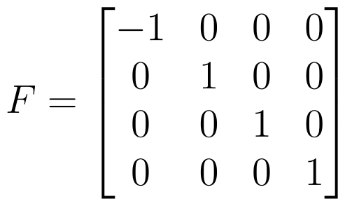
We can use this matrix to flip any dimension since we can combine it with a π radian rotation to flip any two of the signs.

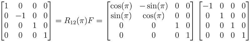
Since this matrix is not parameterized by real numbers, it is discrete.

Euclidean Groups

While we can represent the general transformation in a Euclidean group as

it might be better to represent everything as a linear transformation. Unfortunately, there’s no way to represent a translation with a linear transformation since linear transformations keep the zero vector at the zero vector and translations move the zero vector. Fortunately, there is a way out with homogeneous coordinates. We’re going to represent our 3D points with a 4D vectors with the restriction that the vector has to be “normalized” so that the fourth coordinate is 1.

This “normalization” restriction means that we’re no longer working in the standard Cartesian vector space ℝⁿ, but the real projective space ℝℙⁿ. There is quite a lot you can say about the Real Projective space, but I won’t go into unnecessary detail here. If you want the details, check out eigenchris and sudgylacmoe’s channels.

I also found this video while I was searching for this topic, but I haven’t watched it yet.

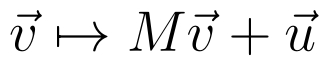
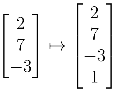
Anyway, for us, all we need to know is that if we have a matrix of the form

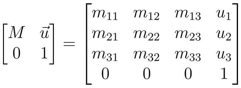
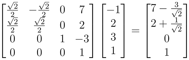
where M is the orthogonal matrix and u is the translation vector, then multiplying our vector by this matrix will get us the rotation and the translation we want. For example, this matrix should rotate π/4 radians counterclockwise around the z-axis and then shift the vectors over by the rightmost column.

To get the Special Euclidean Group, we just restrict M to be an SO(n) matrix instead of a general O(n) matrix.

Rotational Kinetic Energy

While we’ve simplified the description of the system, we haven’t necessarily simplified the equations of motion. Let’s go back to the standard particle Lagrangian (Feel free to try to generalize this stuff to the charged particle Lagrangian, though.).

For this to work as a rigid body, we can treat the rigid body as a combination (and later an integral) of discrete particles (and later continuous mass densities) chosen so that each particle has a mass and distance close to the region it represents.

The (n) means the nth term in the sum. It’s not a covariant index.

Our goal is to convert these interdependent velocity coordinates into 6 independent velocity coordinates. Three of these coordinates should correspond to the position of the rigid body and three of these coordinates should correspond to the orientation of the rigid body. We’re going to work a bit with 2D coordinates along the way, though, to inspire us.

First Attempt

Our first step is to identify the point whose velocity will give us the translational velocity coordinates. Ideally, this point would only experience an acceleration if there is an external force. To figure this point out, we can plug our current Lagrangian into the Euler-Lagrange equations with the potential equal to zero. Unfortunately, this process does not work because it says that all of the points are moving with a constant velocity, which means we’re not rotating.

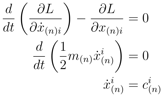
There’s no way to get these particles rotating unless we allow for interactions between these particles, let’s relax our rigid body requirements and work with a stiff body. With a stiff body, we can model each point as being attached to every other point with a stiff set of springs (This model is actually more realistic than a rigid body, but slightly more difficult to study.). The potential energy for such a system is

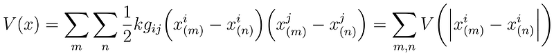
where k is some huge number. We can try to plug the resulting Lagrangian into our Euler-Lagrange equations, but we’re going to have the opposite problem. Every particle can move at a different velocity, but the motion of each particle depends on the position of every other particle. We’ll see if we can come up with a way around it.

Cyclic Coordinates

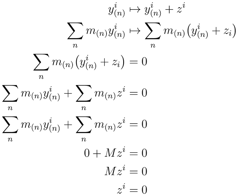
Note that only the difference between coordinates shows up in the Lagrangian. As we discussed in the section Translations, since we’re only looking at differences of coordinates, we can translate the entire system in any way we want without changing the Lagrangian. We therefore have hidden cyclic coordinates. A cyclic coordinate is any coordinate that we can change without changing the Lagrangian. In our case, I’m going to replace all of our current vectors with our vectors plus some vector.

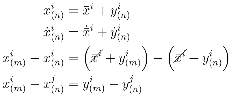
Then, we can plug these equations back into our Lagrangian to get

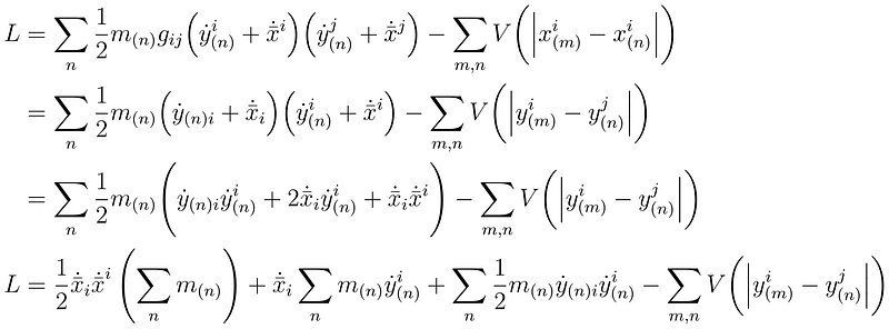
As you can see, the potential (at least the part that depends on the distance between the masses in the system) no longer depends on the x bar variable, which means it’s cyclic. I’m going to make a new variable here so we don’t have to carry the sum of the masses throughout the system.

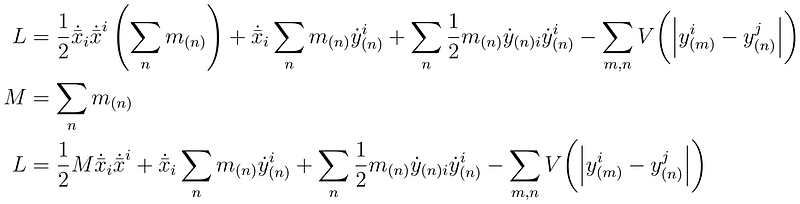
Our Lagrangian still doesn’t look great, but maybe we can plug it into our Euler-Lagrange equations and see if we can’t simplify some terms.

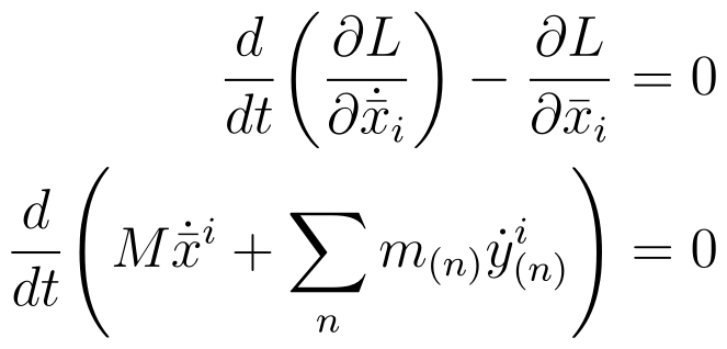
This looks much better, especially since we have some quantity that’s constant in time. We should try to figure out if we can make that quantity look a little nicer. We have a lot of freedom to do so since I’ve specified nothing other than “some point in space,” so we’re going to try to pick a point for x bar that’s manageable. Our first step will be to simplify this expression.

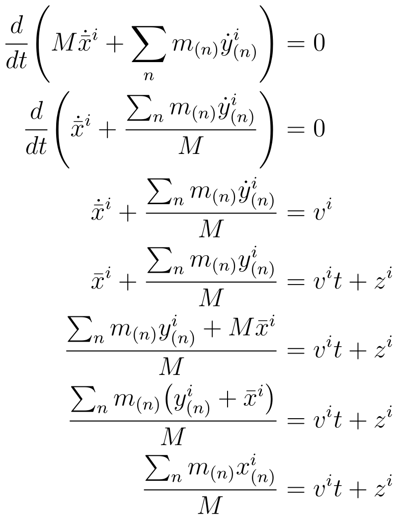
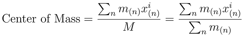
So now, we have this new position variable that moves with a constant velocity. We call this position variable the center of mass.

Now, remember that we have not specified x bar in any way beyond it being a vector that isn’t affected by the potential. In other words, x bar must move with a constant velocity. So if x bar and the center of mass both have to move with a constant velocity, why not set x bar to be the center of mass? If we do, we can see

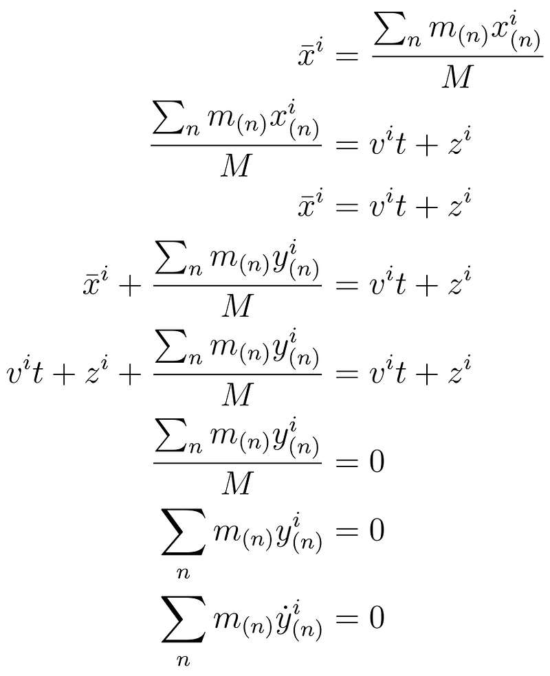
This term shows up in our Lagrangian and it just goes to zero.

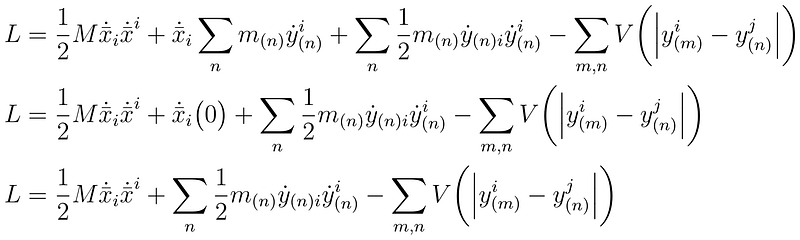
Now, we’ve eliminated all the cross terms. We can also eliminate the potential term since the distance between points is going to be constant so the potential is going to be constant. Later, we’ll be able to add a potential back into the equation that depends on the minimal number of coordinates needed to describe the object.

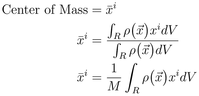
The Integral Form of the Center of Mass

Since we’re almost never working with point masses attached to each other by mystical infinitely stiff massless rods, we’re going to need to convert our center of mass into an integral. We integrate over volumes, so we can divide our mass by the volume to get density.

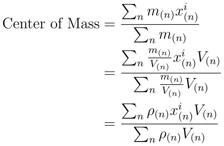
We can then convert the sum to an integral with standard integration arguments.

Shortcut

This entire discussion is Newton’s Second Law. If you wanted to take Newton’s Laws as axioms, then this section would have been a given. In fact, if you wanted to take Euler’s Laws of Motion as axioms, this entire article would be largely redundant.

Incorporating the Rotation

We’ve proven that the center of mass will travel with a constant velocity if we don’t have an external force, but how can that help us? If we didn’t have a rigid body, we would have to stop here or maybe do something with total angular momentum. Here, we need to use the defining property of a rigid body. Since the distance between points doesn’t change in a rigid body, the distance between any point in the rigid body and the center of mass doesn’t change. If we choose a reference frame where the origin is at the center of mass, non-zero translations are no longer possible,

which means the only possible distance-preserving transformations are rotations. We can therefore specify the entire orientation in N dimensions with N(N – 1)/2 coordinates.

Rigid Particle Bodies in 2D

In 2D, we can represent the coordinates of each particle of the rigid body in polar coordinates with the center at the center of mass. This fact means we can write the square magnitude of the velocity as

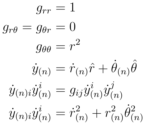
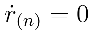
We can then use the rigid body constraints to greatly simplify this expression. First, note that the distance from the center of mass cannot change since that would require a translation and we can only rotate, so

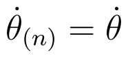
Furthermore, note that every point is going to rotate by just one angle since the number of parameters in SO(2) is 2(2 – 1)/2 = 1. Since each angle is going to change by the same amount, the time derivative of any angle is equal to the time derivative of any other angle.

Plugging everything in gets us

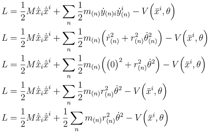
So now, we’re pretty much done. We have reduced the 2 n coordinates needed to describe the system to two translation coordinates and one rotation coordinate. We can only make one more simplification here, and that’s to collect the mass and radius terms into the moment of inertia.

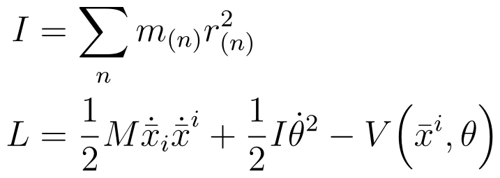
Rigid Bodies in 2D

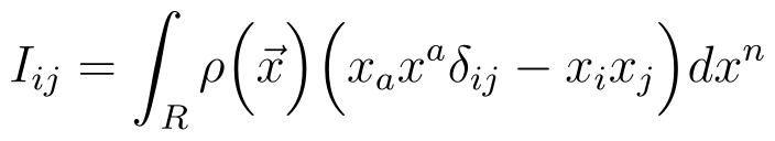
To move to the general system, we again divide the mass by the volume and convert the sum to an integral to get

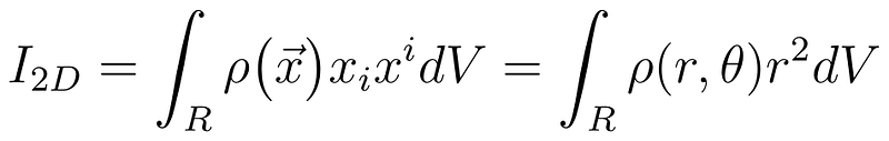
This formula is the moment of inertia for a 2D rigid body. The Lagrangian remains unchanged.

Angular Velocity in 3D

As before, I said that we could represent a rotation by picking an axis, and then doing a rotation in the hyperplane perpendicular to the axis. In 3D, this means that we can specify a vector of unit length for our axis, and then we can rotate in the 2D plane. Since we can do rotations in 2D with one angle, we call this representation of a 3D rotation the axis-angle representation.

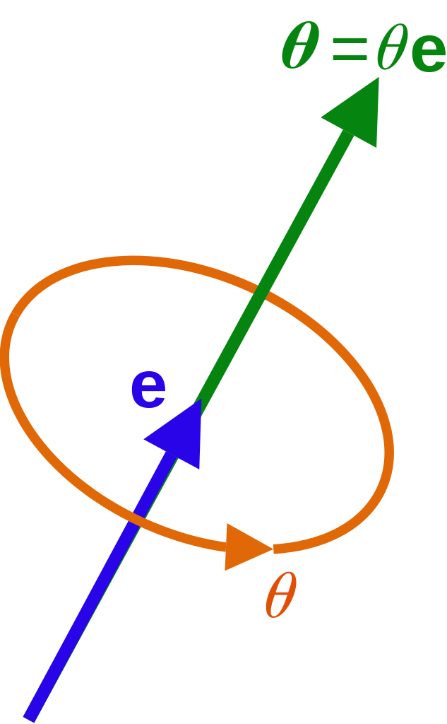
It’s going to be difficult to keep the axis unit-length and we have to figure out how to work with the angle, but we can get rid of all these problems by multiplying our unit length axis by our angle in radians. Doing so makes a lot of things simple because everything is just a vector. You could (and we probably will) represent angular components in terms of matrices, quaternions, etc. depending on the scenario, but pretty much every rotational quantity in Physics is represented in the axis-angle representation in its default form, so we’re going with that.

Rigid Particle Bodies in 3D

With a 2D rigid particle body, we want to somehow use the angular velocity and the position of the particle to figure out the velocity. We can use a few facts to help us and check our math.

v ⋅ rᵢ = 0 since we don’t want the points to move away from the center of mass.
ω ⋅ v = 0 since the angular velocity points along the axis of rotation and and particles shouldn’t be moving relative to the center of mass in the direction of the axis of rotation.
The magnitude of the velocity should be proportional to how fast you’re rotating (the magnitude of the angular velocity) AND how far away you are from the axis of rotation (the magnitude of the part of the position perpendicular to the axis of rotation).
If the position is on the axis of rotation, the velocity should be zero.
The distance traveled by any point after one complete counterclockwise rotation of constant speed must be equal to 2 π r⟂, where r⟂ is the part of r perpendicular to the axis of rotation.

It turns out that these constraints are incredibly restrictive in 3D, which give us a unique relationship. We can use the wedge product and the Hodge star to construct a vector perpendicular to two other vectors.

Alternatively, we could use the cross product.

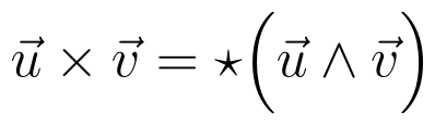
These two expressions are mathematically equivalent, but the cross product is pretty fragile, though, so we’re going to avoid it. In either case, it turns out that the wedge/cross product is exactly what we’re looking for. In fact, the velocity of any point is exactly equal to ⋆(ω∧rᵢ) + v, where v is the velocity of the center of mass, so the y coordinates must be equal to ⋆(ω∧rᵢ). We can plug this expression into our original Lagrangian to get

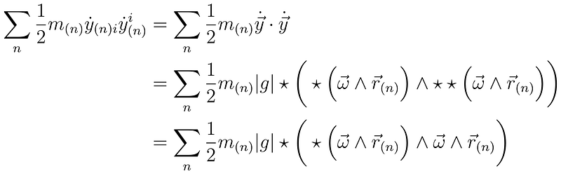
It’s entirely possible that we should have the | g | term in this inner product since you would expect the coordinates to change against the basis vectors.

Note here that we can take inner products between k-vectors or k-covectors by taking the wedge product of a k-(co)vector with its Hodge dual. We can use the ideas from the previous few articles to turn these few difficult to work with things into a lot of things that are easier to work with.

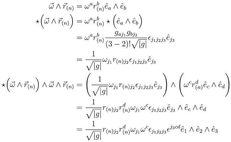
Most of the rules for the expansion comes from the previous article, but we also decided to not enforce any order in the wedge product until the very end, which meant that we had to divide by the factorial term. Furthermore, we also had to introduce an extra Levi-Civita symbol to enforce the order. Lastly, we’re explicitly working in 3D here or else we’d have to deal with multiple basis k-vectors.

We can use the rules for multiplying Levi-Civita symbols to convert them to Kronecker deltas.

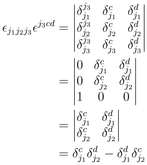
This result simplifies our previous result

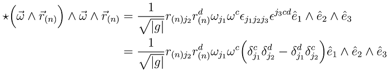
We have two non-zero cases. First, we could have j₁ = c.

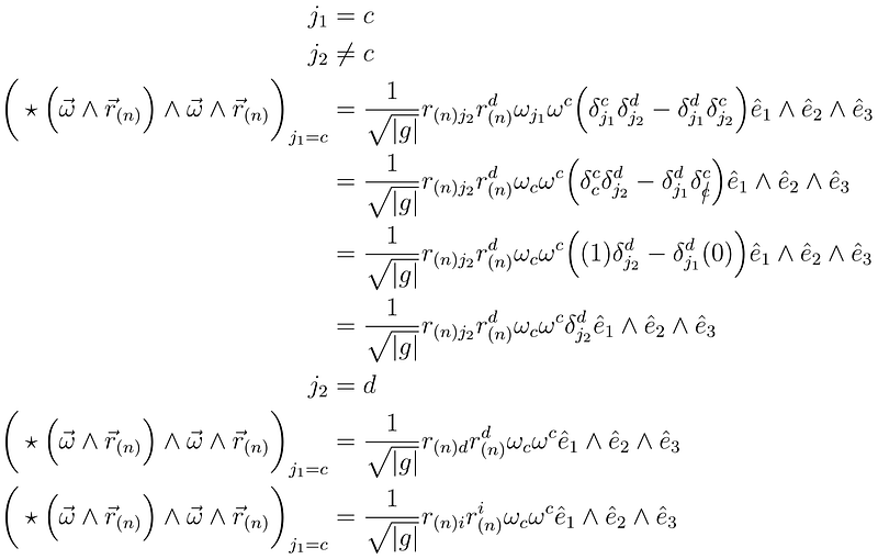
I’ve renamed the index d to the index i because it might cause some confusion later, but you should interpret this line as taking the inner product of each r vector with itself times the inner product of the ω vector with itself. Our second case is when j₁ = d.

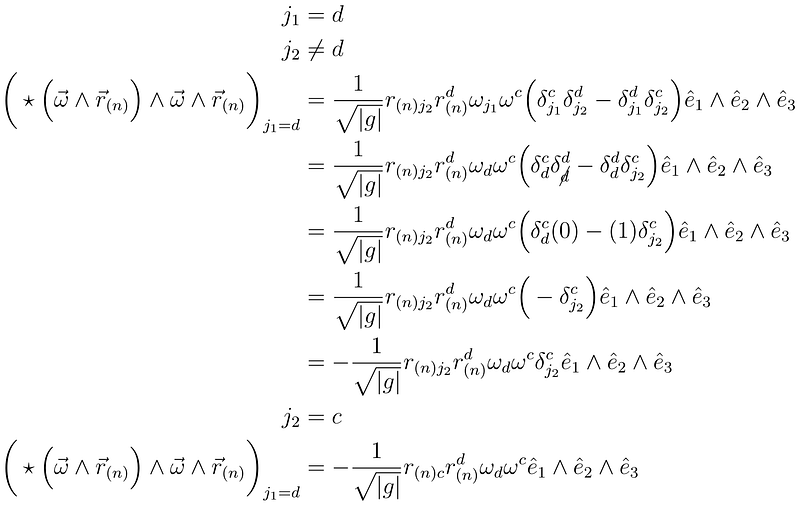
Here, the difference is that we have a minus sign and that the indices are mingling together. We can plug both of them back into our inner product formula.

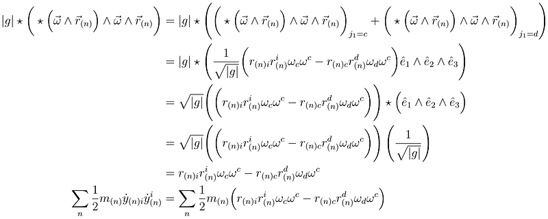
So now, we’ve gotten rid of most of the weird stuff and we’re left with just two kinds of terms. With some clever factoring and a Kronecker delta, we can pull the angular velocity out completely.

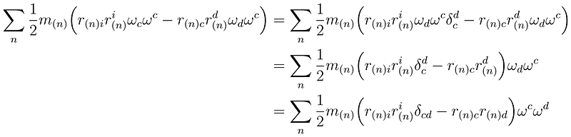
Here, I’ve flipped the d indices using the standard metric tensor raising and lowering indices stuff. Anyway, note that the dynamical variables (angular velocity) and the fixed variables (r and m) are separated. Furthermore, we can pull all the fixed variables into one object known as the inertia tensor.

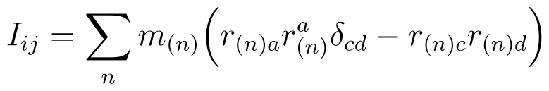
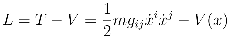
Our Lagrangian then becomes

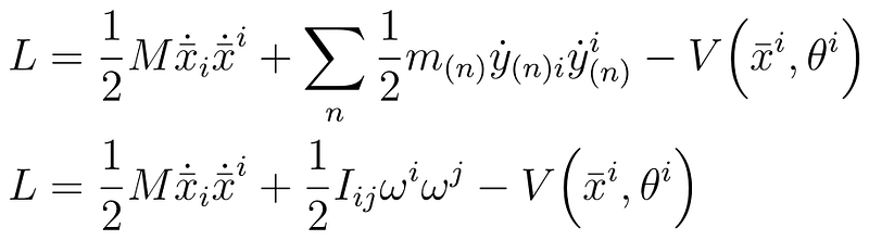
Since the term with the angular velocity and the inertia tensor depends on the velocities of the points and came from the general kinetic energy, we call that term the rotational kinetic energy.

Potential Energy

Since the position of the center of mass (x bar) and the orientation (θ) uniquely determine the position of all the masses, the potential energy must be a function of the center of mass and the orientation.

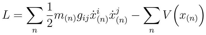
Generalizing to Continuous Media

Again, most objects aren’t point masses attached to each other with rigid massless rods, but we can generalize this approach by converting our sum over a mass into an integral over a density.

Lie Algebras Makes This Process a Lot Simpler, Especially in Higher Dimensions

We’ll cover this topic in a lot more depth later, but we can represent any rotation by exponentiating skew-symmetric matrices, from which the equations of motion just pop out along with the representations of motion.

Principal Axes Frame

While this Lagrangian is valid, it’s not that great to use because the inertia tensor will change as an object rotates. To fix this problem, we can find the inertia tensor in a reference frame that rotates with the object and then convert everything external to the rigid body into that reference frame. Doing so will get a little annoying because we’ll have to add stuff to account for the rotation, so we might as well make it as easy as possible for us. Since the inertia tensor is a real symmetric matrix, we can always diagonalize it, which means we can choose a reference frame in which all the off diagonal elements are zero. This reference frame is known as the principal axes frame.

Euler’s Equations for Rigid Bodies

If we try to put our Lagrangian into the Euler-Lagrange equations, things get difficult and break down. Our inertia tensor is either constantly changing in the world frame or our angular velocity is changing in weird ways in our principal frame. In either case, it’s difficult to get the equations of motion. We can figure it out if we work in the principal axes frame to get rid of the arbitrary coordinates while working in the body frame so we can use the multivariable chain rule. If we do, we’ll get Euler’s Equations for Rigid Bodies, which we’ll cover in much greater depth when we get to Hamiltonian Mechanics. For now, though, I’m just going to leave you here because this article is way too long already.

What’s Next?

We’re going to talk more about rotation in later articles, but we’ll stop here for now. The inertia tensor is a pretty good start for talking about tensors in Classical Mechanics, but it’s far from the only tensor in Classical Mechanics. In the next article, we’ll talk about a whole family of tensors known that show up in the multipole expansion.

Self-Promotion

If you liked this article, you probably know someone else who will. It would help me out if you could share this article with them. If you really liked this article or any of my other articles, you can help me write them by donating to my ko-fi account. If you’re not already a Medium member and you like the articles on the website, you can name me as your referred member and a portion of your monthly fee will help support me. Lastly, if you know of a cool application or idea that relies on topics covered in my articles, let me know in a response, DM, etc.