The Power of Recurrent Neural Networks

…and how they allow us to learn almost any dynamical system given the right data

With four parameters I can fit an elephant, and with five I can make him wiggle his trunk. John von Neumann

Neural networks have come to dominate modern AI Research in recent years, and with good cause: they have provided powerful tools in extracting complex patterns from data, be it when classifying or generating images, aiding in medical diagnosis or processing natural language.

As a short reminder: neural networks are formed by a set of directed units called neurons. These neurons can connect to and pass input between each other, depending on the strength of their respective connections. The sum of the inputs to a given unit is run through an activation function to give its output.

Biological intuitions can come in handy here (although they have their limits): you can think of a neural network as a set of neurons connected via synapses, which either fire or don’t, depending on how much input they receive. The strength of their respective connections determines how much the input from one neuron excites or inhibits the activity of the neuron it is connected, and the activation function determines how and when it fires given the inputs.

While neural networks have shown to be really good at doing a bunch of things, many people (among them me in this article) argue that pure neural networks are, at least to some extent, overrated when it comes to their power to explain our brain and provide the architectural basis for more sophisticated, human-like AI. There are a lot of things they can’t do and won’t be doing any time soon.

But at the same time, neural networks are powerful approximators. Looking into more detail at what neural nets can do in a more formal sense leads us to some fascinating results at the overlap between mathematics and theoretical computer science, with some neuroscientific implications thrown into the mix as well.

The Universal Approximation Theorem

Moving from the two-body problem to the three-body problem, physics students in their second semester usually find out to their horror that almost no real-world problem can be solved analytically.

But luckily there are ways around having to find perfect solutions to difficult problems: approximations with and decompositions into smaller, simpler bits and functions are among the neatest tricks in the mathematician’s and physicist’s cookbooks. The trigonometric functions and the exponential function can be decomposed into polynomials, functions can be Taylor expanded around a point, probability distributions are approximated by Gaussian, numerical methods like the Newton-Raphson method allows us to iteratively find the roots of a function, etc.

As von Neumann notes in his cheeky comment, given enough parameters, and parameters that are sufficiently expressive, you can fit pretty much anything to anything.

And so likewise it can be shown that all functions on a continuous subset of real space can be approximated by combining a set of simple functions. This simple combination of functions needed to approximate any other function can be expressed by a single-layer neural network equipped with the right activation functions.

This theorem known under the name of The Universal Approximation Theorem was shown to hold by Cybenko for the sigmoid activation function, but can also be extended to others, such as the hyperbolic tangent.

Nevertheless, Marvin Minsky and Seymour Papert caused quite the stir when they published their book on the perceptron in 1969, in which they showed that there are a lot of intuitively very simple functions that neural networks can’t approximate, e.g. parity (which relates to the problem that they don’t exist on connected subsets of real space), but as it turns out using deep neural networks with multiple layers does the trick for approximating these kinds of functions as well.

So we can express, under some mild constraints, almost any function we want (given a sufficiently large neural network with enough layers and enough parameters to tune) and use this function to map an input to an output, which is essentially what a function does.

This is already pretty neat. We can fit the elephant. But can we make him wiggle his trunk?

Dynamical Systems Approximation and Recurrent Neural Networks

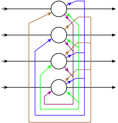
Recurrent neural networks (RNNs) (read here for an overview) are a subtype of artificial neural networks in which a temporal sequence is included, allowing the network to exhibit dynamical behavior (how a system behaves as time is passing).

It was shown in 1993 by Funakashi and Nakamura that the universal approximation theorem extends to dynamical systems as well.

To understand how it can, we need to understand that a dynamical system is characterized by its flow field plus some initial conditions. This flow field determines the derivative of its state variables, and therefore, its behavior in time. This flow field can be written as a function (where the apostrophe after x denotes a derivative…sorry for that but Medium is not really optimized for math equations):

x’(t)=F(x(t))

We can usually discretize these dynamical systems in time, in the sense that we define x at a certain time t+1 through a function on its value at time t and reexpress the flow field through a new function G(x(t)) that takes care of this mapping:

x(t+1)=G(x(t))

The mathematical details of how we move from F(x) to G(x) can be a bit complicated, but the bottom line is that the state of the system at time t+1 depends on the state at time t, sent through this function G. The variable x(t) can be thought of as the value of a unit within the output layer of the recurrent neural network at time t, which you can read out just as in every feedforward neural network.

The dynamics of the system in time then become clear by iteratively applying this mapping again and again:

x(t+2)=G(x(t+1))

If you know the initial state of the system at time t=0, you will know its state at every point in the future t=T, and you will, therefore, have completely characterized the system.

Behold, the elephant is wiggling his trunk.

Learning Dynamical Systems

As Funahashi and Nakamura state, dynamical time-variant systems have “considerable general applications” in all of the sciences. Life is not static, and almost all things worth studying move around and wiggle constantly. The Dow Jones is an observable of a dynamical system. So are tectonic shifts potentially leading to earthquakes.

The examples are infinite, but let’s say we have found a dynamical system in the wild that interests us.

Say we only have some observations x_i at different times t_i, but we are still lacking an understanding of the underlying dynamics of the system, encoded by the function F(x), or respectively G(x).

Notice that this is the state of affairs for pretty much every scientific experiment ever.

Now we can ask the following question from a purely data scientific point of view: how do we learn to explain the data x_i by fitting a model to it without having to analytically figure out what is going on?

The answer follows from everything we discussed so far: we do this by figuring out how the recurrent connections of our network approximate the function G(x) equivalent to the flow field of the dynamical system.

This allows us to encode its entire dynamics within the parameters of the network, which can be learned by the usual machine learning optimization algorithms like gradient descent from the data.

Understanding the Dynamics of the Brain

One of the most well-known and most puzzled-over dynamical systems is the brain. The interactions of neurons form a dynamical system where the intuitive connection to recurrent neural networks seems pretty clear.

But then there are many dynamical subsystems in the brain. Every single neuron, for instance, is in itself is again a complex dynamical system. The Hodgin-Huxley model describes how the firing of a neuron depends on the changing synaptic conductances caused by time dependence of ion flows within the synapse.

But as we can learn any dynamical system with an RNN, this means that we can also use an RNN to learn to model the dynamics single neuron.

Research indicates that many mental illnesses are connected to changes in network dynamics (read here for a great overview), and many useful computational abilities of the brain, such as associative memory, might emerge from dynamical system properties like attractor states (the Hopfield network is an early implementation of this).

Assume, for example, we have brain data, be it FMRI, EEG or single neuron spike trains from healthy patients vs. schizophrenic patients. We can then try to learn the dynamical system underlying the data with a recurrent neural network with machine learning algorithms like the variational autoencoder.

Once we have learned the best model from the data and encoded it in the RNN, we obtain a generative model of the data (I explain what generative models are and why they are so cool in this article). We can then analyze this model in order to improve our understanding of what might cause the changes in network dynamics associated with pathologies like schizophrenia.

Depending on how sophisticated the model is, we can also try to make it biologically interpretable (the problem of explainability is still present in this context, as in many other machine learning applications) in order to extract biologically causal mechanism from the learned model and simulate the effect of novel medical interventions.

Nevertheless, the brain is very messy and complicated, and these approaches are yet tricky to carry out in practice.

But on the other hand, the complexity of the brain indicates that it will be hard to come by analytical descriptions of it, so we need approaches ground in statistics and data science to learn good approximate models.

The approximating power of recurrent neural networks can provide an invaluable tool to do just that.