
The Power of Python: Time-Series Analysis with statsmodels, tslearn, tssearch, and tsfresh
Python Time-Series
Introduction
Time-series analysis is crucial in fields like finance and healthcare, where understanding data patterns over time is essential. In this article, we’ll explore four Python libraries — statsmodels, tslearn, tssearch, and tsfresh—each tailored for different aspects of time-series analysis. These libraries provide powerful tools for tasks ranging from forecasting to pattern recognition, making them invaluable resources for various applications.
Dataset
The dataset employed for this analysis, sourced from Kaggle, provides a comprehensive window into various physical activities through accelerometer data. The activities are divided into 12 distinct classes, each corresponding to a specific physical action, such as standing still, sitting, walking, or engaging in more dynamic activities like jogging and cycling. Each activity is recorded for a duration of one minute, providing a rich source of time-series data. To simplify the analysis and maintain focus, this study exclusively utilises data from a single subject within the dataset, offering a snapshot of their movements and physical activities.
The libraries used for this analysis are:
# statsmodels
from statsmodels.tsa.seasonal import seasonal_decompose
from statsmodels.tsa.stattools import adfuller
from statsmodels.graphics.tsaplots import plot_acf

#tslearn
from tslearn.barycenters import dtw_barycenter_averaging

# tssearch
from tssearch import get_distance_dict, time_series_segmentation, time_series_search, plot_search_distance_result

# tsfresh
from tsfresh import extract_features
from tsfresh.feature_selection.relevance import calculate_relevance_table
from tsfresh.feature_extraction import EfficientFCParameters
from tsfresh.utilities.dataframe_functions import impute
Statsmodels
From thestatsmodels library, two essential functions play a pivotal role in understanding the characteristics of acceleration data collected from the x, y, and z directions.
First, the adfuller function serves as a powerful tool to determine the stationarity of our time-series signals. By subjecting our data to the Augmented Dickey-Fuller test, we can ascertain whether the acceleration signals exhibit a stationary behaviour, a fundamental requirement for many time-series analysis techniques. This test helps us assess whether the data changes over time or not.
def activity_stationary_test(dataframe, sensor, activity):
  dataframe.reset_index(drop=True)
  adft = adfuller(dataframe[(dataframe['Activity'] == activity)][sensor], autolag='AIC')
  output_df = pd.DataFrame({'Values':[adft[0], adft[1], adft[4]['1%']], 'Metric':['Test Statistics', 'p-value', 'critical value (1%)']})
  print('Statistics of {} sensor:\n'.format(sensor), output_df)
  print()
  if (adft[1] < 0.05) & (adft[0] < adft[4]['1%']):
    print('The signal is stationary')
  else:
    print('The signal is non-stationary')
Additionally, the seasonal_decompose function provides invaluable insights into the structure of our time-series data. It decomposes the time series into three distinct components: trend, seasonality, and residuals. This decomposition enables us to visualise and understand the underlying patterns and anomalies in our acceleration data.
def activity_decomposition(dataframe, sensor, activity):

  dataframe.reset_index(drop=True)
  data = dataframe[(dataframe['Activity'] == activity)][sensor]
  decompose = seasonal_decompose(data, model='additive', extrapolate_trend='freq', period=50)
  fig = decompose.plot()
  fig.set_size_inches((12, 7))
  fig.axes[0].set_title('Seasonal Decomposition Plot')
  fig.axes[3].set_xlabel('Indices')
  plt.show()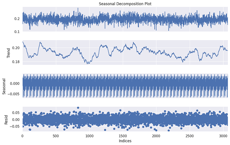
Tslearn
In the context of time-series analysis with the tslearn library, we extract meaningful insights from the x-axis acceleration data captured during walking activities. To begin, we adopted a segmentation approach, breaking down the continuous acceleration signal into discrete segments or windows of a specified length (e.g., 150 data points). These segments offer a granular view of the motion during walking and become the basis for further analysis. Importantly, we employed an overlap of 50 data points between adjacent segments, allowing for a more comprehensive coverage of the underlying dynamics.
template_length = 150
overlap = 50  # Adjust the overlap value as needed
segments = [signal[i:i + template_length] for i in range(0, len(signal) - template_length + 1, overlap)]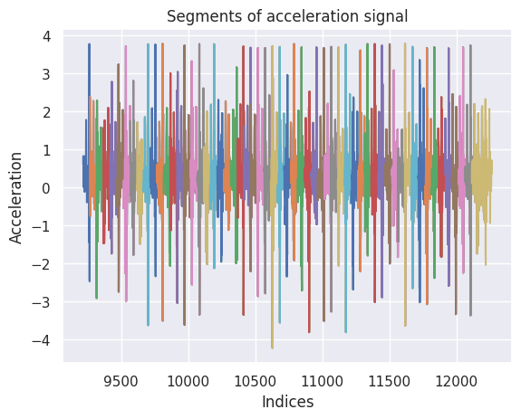
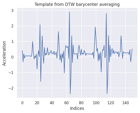
To derive a representative template that encapsulates the typical characteristics of walking from these segments, we turned to the dtw_barycenter_averaging function. This method employs Dynamic Time Warping (DTW) to align and average the segmented time series, effectively creating a template that captures the central tendencies of walking motion.
template_signal = dtw_barycenter_averaging(segments)
template_signal = template_signal.flatten()
The resulting template provides a valuable reference for subsequent classification and comparison tasks, aiding in the recognition and analysis of walking activities based on x-axis acceleration.
Tssearch
When using the tssearch library, we used the time_series_segmentation function that takes a time series, a configuration for distance metrics, and a template signal as input. It uses dynamic time warping (DTW) or other similarity measures to identify segments within the input time series that are most similar to the provided template signal.
The primary goal of this function is to locate and extract segments of the input time series that closely match the template signal. These segments are found by comparing the template signal to the input time series, and the function returns the positions or indices in the input time series where these segments begin.
segment_distance = get_distance_dict(["Dynamic Time Warping"])

segment_results = time_series_segmentation(segment_distance, template_signal, signal_np)

for k in segment_results:
  plt.figure(figsize=(15, 3))
  plt.plot(signal_np, color='gray')
  plt.vlines(segment_results[k], np.min(signal_np)-1, np.max(signal_np) + 1, 'C1')
  plt.xlabel('Indices')
  plt.ylabel('Amplitude')
  plt.title(k)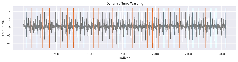
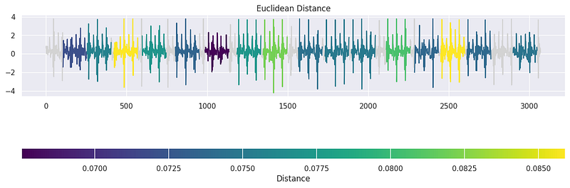
Another function from the tssearch library used to uncover similarities and dissimilarities within time-series data. To begin, we configured a dictionary, dict_distances, to specify the distance measures for our search. Within this dictionary, we defined two distinct approaches. The first, labeled 'elastic,' employed Dynamic Time Warping (DTW) as the similarity measure. We customised DTW with specific parameters such as dtw_type set to 'sub-dtw' and alpha set to 0.5, allowing for flexible alignment and comparison of time series. The second approach, 'lockstep,' utilised the Euclidean Distance to measure similarity in a more rigid manner. With these distance configurations in place, we executed a time-series search using the time_series_search function, comparing a template signal to the target signal (signal_np) and specifying an output of the top 30 matches.
dict_distances = {
    "elastic": {
        "Dynamic Time Warping": {
            "function": "dtw",
            "parameters": {"dtw_type": "sub-dtw", "alpha": 0.5},
        }
    },
    "lockstep": {
        "Euclidean Distance": {
            "function": "euclidean_distance",
            "parameters": "",
      }
    }
}

result = time_series_search(dict_distances, template_signal, signal_np, output=("number", 30))
plot_search_distance_result(result, signal_np)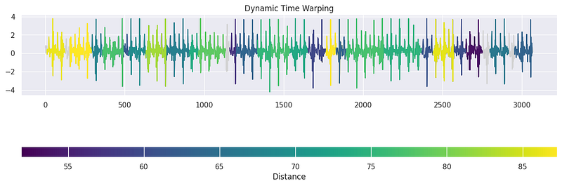
Tsfresh
The tsfresh library proves to be a great tool for automating the process of feature extraction. To initiate this process, we defined a set of extraction settings using EfficientFCParameters(), which specifies the feature extraction parameters and configurations. These settings allow us to control which features are computed during extraction. Next, we applied the extract_features function to our time-series data, represented as final_df. We indicated that the 'Activity' column should be treated as the identifier column and provided the feature extraction parameters. Importantly, the library handles the automatic removal of features containing missing values (NaN) through imputation, ensuring a clean and reliable feature set. The result, X_extracted, represents an extensive collection of features extracted from the time-series data. To enhance clarity and accessibility, we converted the result into a Pandas DataFrame, making it easy to explore, manipulate, and integrate these features into our subsequent classification tasks. tsfresh simplifies the often complex and time-consuming process of feature engineering, offering a valuable resource for time-series analysis.
extraction_settings = EfficientFCParameters()
X_extracted = extract_features(final_df, column_id='Activity',
                      default_fc_parameters=extraction_settings,
                      # we impute = remove all NaN features automatically
                      impute_function=impute, show_warnings=False)

X_extracted= pd.DataFrame(X_extracted, index=X_extracted.index, columns=X_extracted.columns)

values = list(range(1, 13))
y = pd.Series(values, index=range(1, 13))

relevance_table_clf = calculate_relevance_table(X_extracted, y)
relevance_table_clf.sort_values("p_value", inplace=True)
relevance_table_clf.head(10)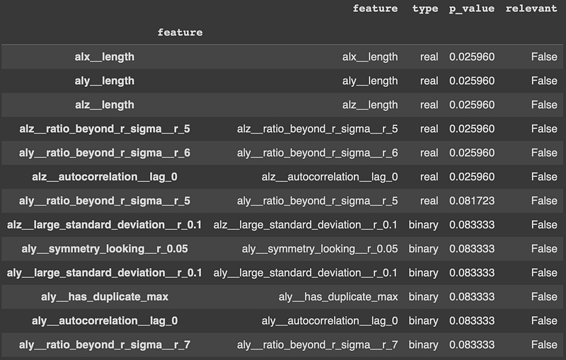
  top_features = relevance_table_clf["feature"].head(10)
x_features = X_extracted[top_features]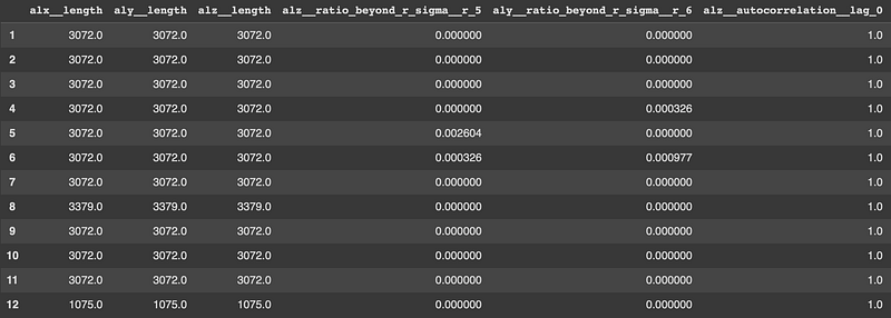
Conclusion
In summary, this article introduced you to the world of time-series analysis and four essential Python libraries: statsmodels, tslearn, tssearch, and tsfresh. Time-series analysis is a crucial tool in various fields, like finance and healthcare, where we need to understand data trends over time to make smart decisions and predictions.
The key takeaway is that each library specialises in different aspects of time-series analysis, and the one you choose depends on your specific problem. By using these libraries, you can tackle a wide range of time-dependent challenges, from predicting financial trends to classifying activities in healthcare. When you start your own time-series analysis projects, remember to explore these libraries to unlock valuable insights hidden in your data, making better decisions and predictions in your field. Time-series analysis is a fascinating and evolving field, and these libraries are your trusted companions on this analytical journey.


