The Power of Precision

Precision is one of those concepts that is not really taught in standard econometric or data analysis classes. But as long as we are using data, it is present at the very heart of all the analysis we do. In this guide, we will learn about precision, what it is, why is it important, and how it affects our day-to-day data work.

So what is it? Precision deals with how we store our variables and perform operations — add, subtract, multiple, divide — across them. While Stata performs all calculations at the highest level of precision, the information that is saved back into the dataset can have lower levels of accuracy. You might have seen storage types, e.g. integers, floats, long, double, and strings, show up on screen. They display the level of detail that exists for each variable. These storage options are also set when we generate new variables or import data. And if we do not specify the storage type, Stata makes a judgement call on our behalf. Most of the time these choices are fine, but they might not be the best under certain circumstances. But if some storage types are always considered more accurate than other, then why don’t we always go for the best option? Because, even though higher precision implies better accuracy, it also means more memory usage, which scales up with the size of the data and the complexity of the operations. Therefore a blanket use of the best storage method is also not advisable. At the end of the day, we need to make smart decisions about precision types while we are doing our data work. This is especially true for Stata, which does not force us to define the precision levels for variables, something that is a norm in some programming languages.

As casual users, we tend to overlook the precision options but as programmers ignoring them can completely change the final results to the point of making them fairly inaccurate. In this guide, we will go over five everyday examples where precision really matters. These deal with routine tasks like if conditions, locals, loops, summations, and unique ids. At the end of the guide, the readers should be well aware of where problem can exist and their potential solutions. Additional reading material is provided at the end of the guide for a deeper dive.

A general note: while all examples presented here are for Stata, the problem itself is not unique to Stata. It exists across all programming languages since precision deals with how computers handle numbers, that is in a binary system.

A brief introduction

Let’s start by highlighting the two main variable types we usually work with in Stata: string and numerical or real variables. If you check the entry help data types in Stata, you can read the details, but here is a quick summary:

Strings are stored based on their length, where the length is defined as follows:

String
    storage       Maximum
    type          length         Bytes
    -----------------------------------------
    str1             1             1
    str2             2             2
     ...             .             .
     ...             .             .
     ...             .             .
    str2045         2045           2045
    strL            2000000000     2000000000
    -----------------------------------------

Stata determines the size of the string based on length of the largest value in the variable. Variables with a very large number of string characters are not optimal to have in datasets, unless you are dealing with text data, e.g. for natural language processing (NLP) applications or similar. They should be converted to numerical variables with value labels where possible. There are also other ways to optimize string variables, but we will leave this for another guide.

Numerical or real variables, in contrast, come in five different flavors — byte, int, long, float, or double — where each has its own level of accuracy:

Screenshot from Stata: `help data types`

The storage types, byte and int are used for standard numbers like 1, 2, 3, 4 that require the least possible space. Note that an integer does not have to stored as an int. The type long is used for large integers that requires more storage space than an int. The last two options, float and double deal with very large numbers, and more importantly, decimal points. Floats have seven digits of accuracy, while doubles have 16 digits of accuracy. We will see later why this makes a difference.

Just to provide a bit of a background, floating points are numbers in scientific notation: 1.23 * 10⁷, or 4.56 * 10^-8, etc. The term float itself refers to the decimal point, whose position can vary between the digits, hence it is floating around. Floats are used for optimizing calculations of very large (e.g., size of galaxies) and very small numbers (e.g., size of atoms). This also makes life easy especially if we are multiplying these two extreme values. For example, multiplying 1.23 x 4.56 and dealing with decimal points later is easier than multiplying the full numbers with all their digits. Such calculations were important in the early computing days when there was limited computational power and very small memory storages. Overtime, different rules have appeared for dealing with the floating point but currently IEEE 754 is the main industry standard.

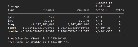
It can get a lot more technical here, so do check out the links at the end of this guide if you want to read more. But in summary, floating points in Stata come as float and double where floats are less precise then doubles by a significant amount:

Storage
     type             minimum                maximum
     -----------------------------------------------------
     float     -3.40282346639e+ 38      1.70141173319e+ 38
     double    -1.79769313486e+308      8.98846567431e+307
     -----------------------------------------------------
     In addition, float and double can record missing values 
     ., .a, .b, ..., .z.

If we do not specify the storage type of numerical variables, then Stata will make an educated guess on our behalf, which might be the wrong option. This is especially true for new empty variables that are usually labeled as floats since Stata does not know if we are going to use them for high precision calculations. Even though Stata does all calculations in double precision (or even quad precision in Mata), which is the highest level of accuracy, if the storage type is wrongly defined, then the precision is lost when the variable information is written back to the dataset. In some cases, this can result in errors that are carried forward through the rest of the calculations. Below we look at five everyday cases in which this can happen.

Case 1: additions and if conditions

Let’s start with a classic example. What do we get when we add 0.1 + 0.2. The answer is fairly simple. We get 0.3. We can also use Stata as a calculator and check this:

di 0.1 + 0.2

and it will spit out .3 on the screen.

Now let’s try and store this information in Stata as variables:

clear

set obs 1
gen x1 = 0.1
gen x2 = 0.2
gen x3 = x1 + x2

now open the browser window by typing br and check what you have:

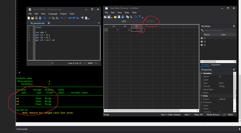
Here we see the first issue. In the browser window it says 0.3 but if you highlight the cell it says .300001, which is not really 0.3. If we describe the dataset, we can also see that all numbers are stored as floats.

Now let’s check the variables we generated ourselves, that are x1 and x2:

count if x1==0.1
count if x2==0.2

Both should theoretically return one observation, but it returns nothing! This is because 0.1 or 0.2 are not stored as exactly those values in the memory. A computer uses a binary system which is just zeros and ones. In this system, there is no exact equivalent for 0.1 or 0.2. In fact, what we consider well defined easy-to-handle decimal numbers have this problem. So the above example is not an error in the software, the computer is trying its best to approximate what we consider are very precise numbers. And this is where floating points come into play. In the words of William Gould, the president of StataCorp, computers are simulating numbers, and simulations are not the reality.

We can circumvent this problem by typing:

count if x2==float(0.2)

And it should now find our case. But this is not really a good solution since this is cumbersome to type every time. We can also just go for higher accuracy by using the double option when generating the variables:

drop x*
set obs 1

gen double x1 = 0.1
gen double x2 = 0.2
gen double x3 = x1 + x2

and now check:

count if x1==0.1
count if x2==0.2

Here the output window will correctly show one observation for each case since the conditions now match perfectly. But now let’s check the last variable, x3, that we generated as a double from our other two double variables:

count if x3==0.3

and we still cannot find that exact value! Even adding two double values is not a good enough approximation to give us a close enough approximation for 0.3.

This can have huge implications for your datasets especially if you are using variables with decimals values as conditions. In our above example, if we type:

count if x3>0.3

Then it will find the value as greater than 0.3. Because even in double precision, there is some small digit attached at the end of a very long decimal space. Let’s check this:

display %20.17f x3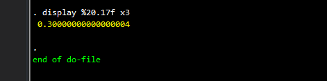

And here we see it the issue. If you are not aware of precision issues, you will mostly likely also not check this by stretching the format command to its limits. This is extremely problematic, especially if you wanted all the values less than or equal to 0.3. If we type

gen dummy = 1 if x3 <= 0.3

we essentially end up with nothing in our one observation example. And if you are applying such filters on a very large dataset, there is a very good chance of skipping or wrongly assigning conditions without even noticing it.

A good way to circumvent this is to avoid doing very precise conditions in decimals and simply moving to the whole numbers or integers range, for example by multiplying the number by 10 or a 100 and rounding it off:

gen x3_2 = round(x3 * 10)
count if x3_2==3

Once we are in the integer range, we are safer.

This can be very sub-optimal, but in general, this is not a Stata-specific problem. Plus, this is not a problem to begin with if you understand numerical storage, because that is how computers have been designed. You can read more about this in Stata by typing help precision. But the important lesson here is that be very careful in dealing with decimal values. And here we just discuss additions. Subtractions can result in much larger precision errors and should be treated with even more caution.

We can generate everything as double, which has a much higher level of accuracy at the expense of storage capacity. For smaller datasets, say less than 5000 observations on modern computers, it should be fine if you double everything. You can even make it the default by setting the option set type double or set type double, permanently but as we saw above, some margin of error is always there.

Case 2: Locals

We use locals often to speed up our calculations since they just exist in the memory. A very good example is the use of the summarize command that gives us mean, minimum, maximum, percentiles values, etc., of variables. But a very common mistake (that I also make), is that most of the time people end up using the less precise option. Let me explain it through an example:

clear

set obs 10
set seed 1000
gen double x = runiform()

We specify the seed for replicability and it is not really needed for this example. If we summarize the variable:

summ x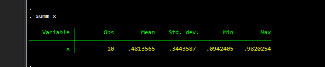

we can see the (rounded) minimum and maximum values are 0.0942 and 0.9820 respectively. We can also see what the stored locals are by typing:

return list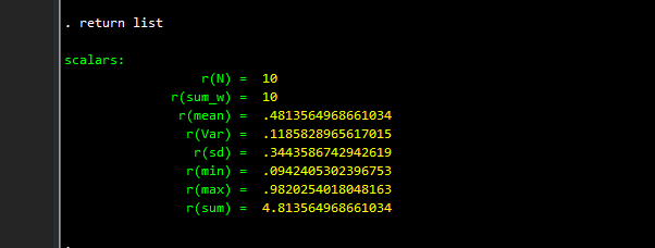

which gives us the list of summary statistics stored in locals that we might want to use. We can try and recover these values:

list if x==`r(max)'

This works perfectly. But:

list if x==`r(min)'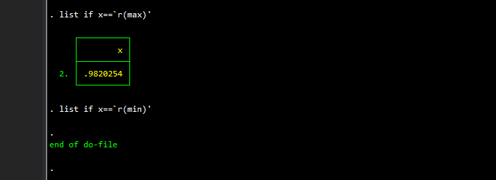

does not! Why is this the case? Essentially the locals in the quotes `r(max)' and `r(min)' are rounded-off string representations of the stored values. The correct option would be to type:

list if x==r(min)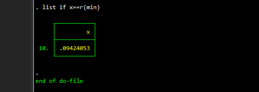

without the quotes, which gives us the values we need. This is extremely important in programs, and loops, and/or doing calculations over a large variable set. One might tend to overlook this because the statement list if x==`r(min)' might not fail in all circumstances, and you would go on assuming that this option works correctly for all the cases and can end up skipping certain values.

Case 3: Summations

I use totals and running sums quite a bit in my guides. Scripting most of the guides was probably the first time that I realized how much precision make a difference. Let’s start with a simple day-to-day example, before I illustrate the problems I experienced in my own applications.

Example 1

We load the system-provided auto.dta dataset and keep two variables:

clear
sysuse auto

keep gear_ratio foreign
sort foreign gear_ratio

If you view the data, you will see that the variable gear_ratio has two decimal points:

. list in 1/10

     +---------------------+
     | gear_r~o    foreign |
     |---------------------|
  1. |     2.19   Domestic |
  2. |     2.24   Domestic |
  3. |     2.26   Domestic |
  4. |     2.28   Domestic |
  5. |     2.41   Domestic |
     |---------------------|
  6. |     2.41   Domestic |
  7. |     2.41   Domestic |
  8. |     2.43   Domestic |
  9. |     2.47   Domestic |
 10. |     2.47   Domestic |
     +---------------------+

What we want is to sum up the gear ratio by the variable foreign, which takes on two values “Foreign” and “Domestic”. Let’s do this calculation using the float and the double options:

bysort foreign: egen        total1 = sum(gear_ratio)  
bysort foreign: egen double total2 = sum(gear_ratio)

// and their shares
gen share1 = gear_ratio / total1
gen share2 = gear_ratio / total2

Here we generate the totals for the gear ratio by each foreign category. Then we calculate the share of each value in the total of that category. We can also browse the values here and compare share1 and share2. They look the same when eyeballing.

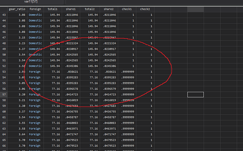
But just to be safe, let’s generate the sum of the shares, which by definition should add up to one for each category:

bysort foreign: egen check1 = sum(share1)
bysort foreign: egen check2 = sum(share2)

And here we notice that without the double option, the Foreign category actually does not add up to 1 but rather 0.999999:

We can also check where this error happens by taking the different between the share values:

gen double error = share2 - share1

and we can see that the margin of error is extremely small and not discernable by just looking at the data.

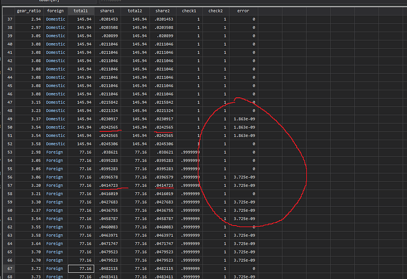
Moreover, there are more errors in the Foreign category, as opposed to the Domestic category, which results in this imprecise adding up.

Example 2

Now let’s talk about where I have encountered precision problems. I have a bunch of guides on polar plots, which essentially deal with laying out the data in a circular format. Since a circle is 360 degrees, or 2 * _pi in Stata, the points and the labels should fully complete the circle.

An important point to highlight here is that Stata does not deal with full circles. It deals with two semi-circles, the top half and the bottom half. This implies that different conditions have to be defined for the top and the bottom halves. Therefore, the combination of halves, and rotation calculations, that are done on the left and the right halves, imply that the four quadrants have their unique case-specific conditions. Therefore, the points on the circles have to be assigned to the right quadrant, and this is where the problem arises.

Let’s see the issue with an illustration. We take the auto.dta dataset again, and let’s say we want to plot the price variable in a circle:

clear
sysuse auto

keep make price
sort price

We sort the data from lowest to the highest price. For each data point, we assign an angle on the circle. Let’s do this with and without the double:

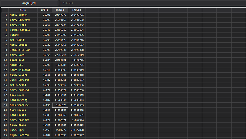
cap drop angle*

gen        angle1 = _n * 2 * _pi / _N
gen double angle2 = _n * 2 * _pi / _N

Here we are dividing the 360 degrees or 2*_pi into _N angles, where each observation has the _n/_N share in 360 degrees.

If we eyeball the data here, the differences are very visible. This is not so surprising since we are dealing with the multiplication of two fractions _n/_N and _pi where the role of precision is very obvious here:

We can now convert the price variables to polar coordinates. Again without going too much in the details, this is done as follows:

// float
gen        x1 = price  * cos(angle1)
gen        y1 = price  * sin(angle1)

// double
gen double x2 = price  * cos(angle2)
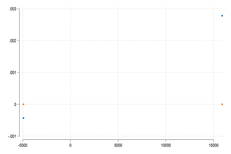
gen double y2 = price  * sin(angle2)

If we plot these:

twoway scatter y1 x1 || scatter y2 x2, aspect(1) legend(order(1 "Float" 2 "Double"))

we can see the two variables completely overlap, at least to the human eye:

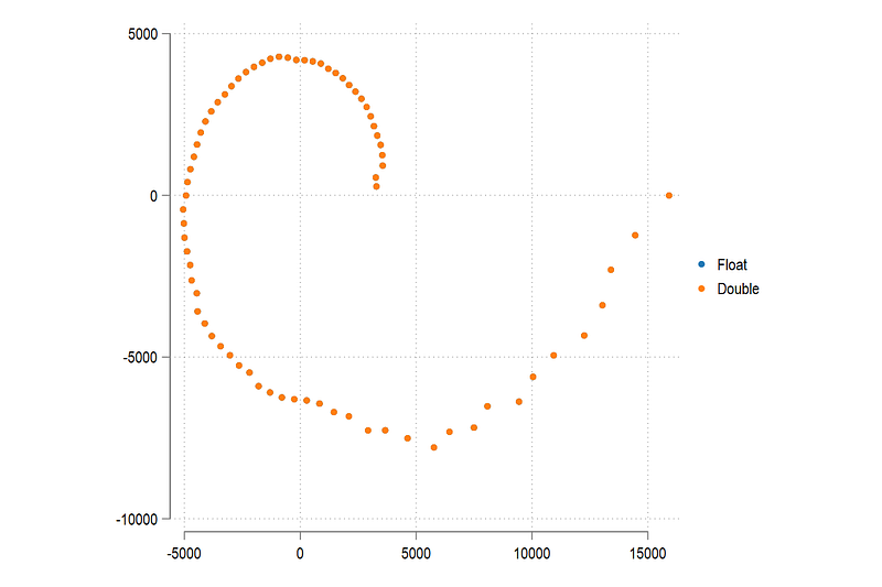
So at this point, one would say, why bother with precision? But let’s keep going.

Now let’s assign each point to a quadrant for which we need additional calculations:

// float
cap drop quad1
gen quad1 = .  
 replace quad1 = 1 if x1 >= 0 & y1 >= 0 
 replace quad1 = 2 if x1 <= 0 & y1 >= 0   
 replace quad1 = 3 if x1 <= 0 & y1 <= 0
 replace quad1 = 4 if x1 >= 0 & y1 <= 0

// double
cap drop quad2
gen quad2 = .  
 replace quad2 = 1 if x2 >= 0 & y2 >= 0 
 replace quad2 = 2 if x2 <= 0 & y2 >= 0   
 replace quad2 = 3 if x2 <= 0 & y2 <= 0
 replace quad2 = 4 if x2 >= 0 & y2 <= 0

and now we compare the two:

gen myerror = 1 if quad2 != quad1

We can see that the last observation in the float variable actually extends beyond the full rotation of one circle and starts a new circle. It is therefore wrongfully assigned to the first quadrant (top right), as opposed to the fourth quadrant (bottom right):

And this is not the only error. If we plot the myerror variable:

twoway ///
 (scatter y1 x1) ///
 (scatter y2 x2) ///
 if myerror==1, ///
 legend(off)

We can see that for the float variables, the two points that are supposed to lie on the horizonal axis, overshoot and end up in the wrong quadrants.

While the overshoot here is extremely small in terms of values, it affects the calculations later on since the values are assigned to the wrong quadrants and therefore we end up using wrong transformations for all calculations later on.

So when dealing with group-wise summary statistics, especially totals, be very careful and preferably use double variables for storing results if you are unsure.

Case 4: Loops

Looping through non integer values is not uncommon but it is highly problematic. Nick Cox even wrote an article on this. This is something I also deal with regularly in my own work. For example, in climate economics, a lot of estimation is done around RCP scenarios that take on values of 2.6, 4.5, 6.0, 8.5 representing different futures, where estimations for different variables come from different policy runs. A variable like this would entail just taking the different variable levels (four in total) and looping over them:

// pseudo code

levelsof rcp, local(lvls)

foreach x of local lvl {
  do something if rcp==`x'
}

This setup is highly problematic and we will see why in a bit. Let’s start with a simple example:

forval i = 0(0.5)1 {
 display `i'
}

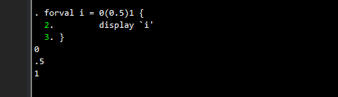
Here we loop from 0 to 1 in steps of 0.5. In total these are three values: 0, 0.5, and 1, which Stata correctly finds. Now let’s reduce the step size to 0.05:

forval i = 0(0.05)1 {
 display `i'
}

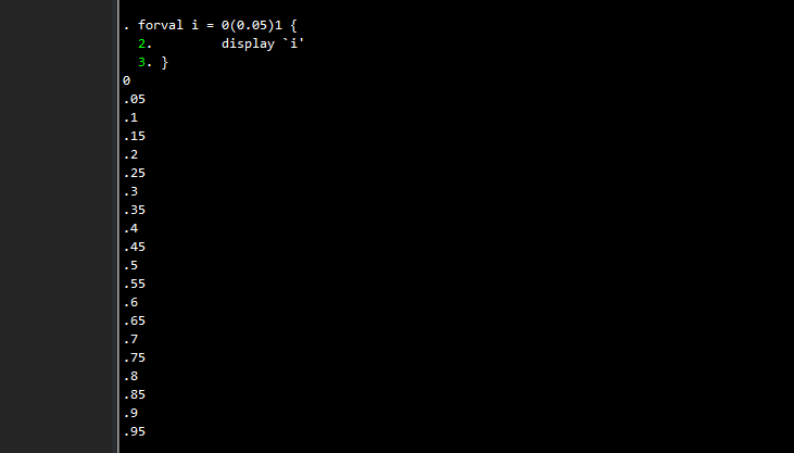
This should give us 20 categories. But in the output, the last category is missing! In other words, the loop skips the value where i should be equal to 1. Here the rounding of the floats have come into play. In each step of the loop, Stata takes on the previous value and adds the step size to it. For example, the first iteration is 0, the second is 0+0.05, the third is 0+0.05+0.05, and so on. Since these are well-defined decimal numbers, the summations compound the binary additions floating point errors, such that by the time we reach the last value, some threshold is crossed that prevents the last value to be recognized as 1.

This does not happen if we use whole numbers, or integers instead:

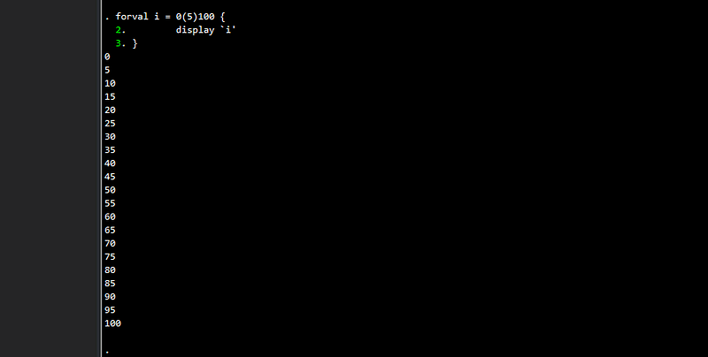
forval i = 0(5)100 {
 display `i'
}

Here we get the complete series where we are not dealing floating point issues:

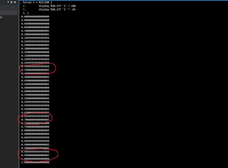
If we try and convert these whole number into decimal points through two methods: (a) divide by 100, and (b) multiply by 0.01, which in theory should be equal, even then, we get different numbers:

forval i = 0(5)100 {
 display %20.17f `i' / 100  
 display %20.17f `i' * .01
}

All of this makes it frustrating when doing seemingly ordinary calculations! Since I also use Mathematica a lot for economic modeling, I have encountered this issue there as well, even though it has one of the most powerful solvers, and provides a fairly large control over precision thresholds.

Here a good suggestion would be to completely avoid looping over decimal values and stick to integers. Make sure that your data has values like 1, 2, 3, 4 that can you label as whatever decimal values you want. But if you are given categorical variables in decimal values, then carefully convert them into numerical wholes through recoding or encoding the variables.

In general, and very broadly speaking, the size of the error is the smallest around the 0. Therefore, try and keep the variables in the +-1000 range, and where possible, as whole numbers or integers. Moving farther away from this range will increase floating point errors, and therefore the accuracy of the results. Again these errors are extremely minuscule and within acceptable tolerance levels, but not advisable for operations that require us to match exact values or assign variables to categories.

If you keep these two points in mind, you will avoid making unnecessary calculation errors, and subsequently will have to deal with less headaches.

Case 5: Long numbers

Another issue with numerical variables that is fairly common are the use of long identifiers, for example, in large surveys or census-level data. In such datasets, usually a unique id is generated at a person level that is a combination of higher level ids. This allows the number to be retraced back to the original components. For example an id like 864220400501 could be some region 86, sub-region 42, block 204, household 005 and person 01. This is a made up number, but it is not unusual to have this type of information.

Let’s input this manually in our dataset with an increment of 1 for subsequent values:

clear

input  x1      double x2    str12 x3
  864220400501 864220400501 864220400501
  864220400502 864220400502 864220400502
  864220400503 864220400503 864220400503
  864220400504 864220400504 864220400504
end

The first one is the default float, the second one we declare as a double, and the third one is a string that we define to be of length 12 characters.

Let’s see what they look like by typing list or checking them in the browser br. And we get something like this:

     +-------------------------------------+
     |       x1          x2             x3 |
     |-------------------------------------|
  1. | 8.64e+11   8.642e+11   864220400501 |
  2. | 8.64e+11   8.642e+11   864220400502 |
  3. | 8.64e+11   8.642e+11   864220400503 |
  4. | 8.64e+11   8.642e+11   864220400504 |
     +-------------------------------------+

It is not unusual to see this type of output since we have not formatted the data. The only variable that is showing correctly is variable x3, since the string length is the format here. Let’s fix the format of the first two:

format x1 x2 %12.0f

and let’s look again by typing list:

. list

     +--------------------------------------------+
     |           x1             x2             x3 |
     |--------------------------------------------|
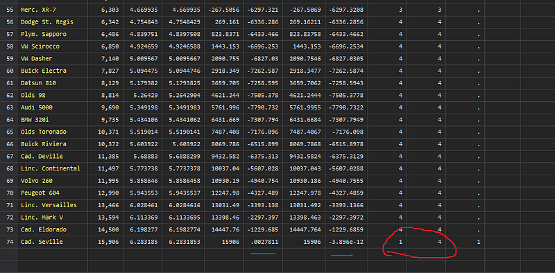
  1. | 864220413952   864220400501   864220400501 |
  2. | 864220413952   864220400502   864220400502 |
  3. | 864220413952   864220400503   864220400503 |
  4. | 864220413952   864220400504   864220400504 |
     +--------------------------------------------+

And here we see the obvious problem. The float has hit its limit for long numbers. It has managed to display the first seven digits correctly (the accuracy level for floats), and after that it is just junk! The double variable x2 shows this correctly and so does the string variable x3. But strings take up more memory and for very large datasets this can be hamper performance.

If your data contains some identifier series that starts with relatively small values and goes up to very large ones, then it is very easy to overlook this floating point limit and end up with wrong ids for higher values. And if you perform operations by identifiers, then the results will also be wrong.

Just be aware that if your unique ids, or other variables have more than seven digits, declare them as long or double to avoid running into calculation errors. If the digit length is more than 16, then good luck keeping up the accuracy! Here I would suggest to just sticking to a string format.

About the author

I am an economist by profession and I have been using Stata since 2003. I am currently based in Vienna, Austria where I work at the Vienna University of Economics and Business (WU) and the International Institute for Applied Systems Analysis (IIASA). You can see my profile, research, and projects on GitHub or my website. You can connect with me via Medium, Twitter, LinkedIn, or simply via email: [email protected]. If you have questions regarding the Guide or Stata in general post them on The Code Block Discord server. We can also collaborate via UpWork.

The Stata Guide releases awesome new content regularly. Subscribe, Clap, and/or Follow the guide if you like the content!