
The Power of A/B Testing
A visual summary of how sample size, effect size and significance level affect the power of A/B testing

A/B testing involves multiple concepts which can be difficult to wrestle with, especially during high-pressure environment such as job interview. So I decided to write this post to clear things up. This post begins with a short technical review of power, two example problems, and extensive visualization that illustrates its interaction with other variables.
This is not an introductory article on statistical testing, to which I have very little to contribute. But if you’re an analyst or data scientist rusty on basic concepts, or product managers who want to acquire some technical savvy on the subject, this is a good review (part of the reason I’m writing the post is to make a visual cheatsheet that I can quickly reference to later on). By the end of the post, you should understand the following concepts:
- alpha: false positive rate; or significance level; or type I error.
- beta: false negative rate; or type II error.
- power: true positive rate; 1 - beta.
- 1 - alpha: true negative rate.
Concept Review
When people talk about alpha and beta, they talk as if the two concepts are apple and orange that can be placed on the same table. In fact, they cannot coexist in the same reality. Alpha controls the false positive rate, in which case we reject null when we should not. Beta controls the false negative rate, in which case we fail to reject null when we should.
Why does this matter? Because power is defined as 1 - beta, it only makes sense to talk about power when the null is false. If you’re already dizzy, here are two pictures to help memory. Both pictures illustrate two-tailed test.
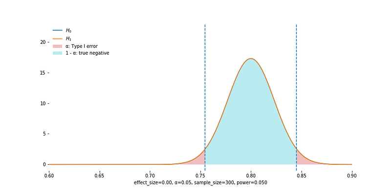
When Null Hypothesis is True
The empirical sampling distribution is the same as the one under the null hypothesis. We are right if we do not reject the null, which happens with probability 1 - alpha (shaded in cyan). The two tails shaded in red have total area equal to alpha, which is the probability we reject null by mistake.
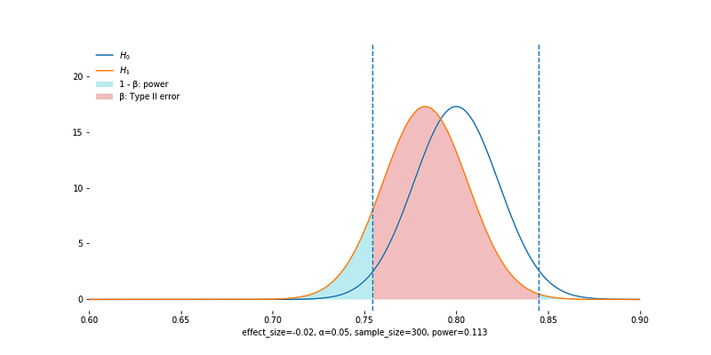
When Null Hypothesis is False
The empirical sampling distribution is different from the one under the null hypothesis. We are right if we reject the null, which happens with probability 1 - beta (shaded in cyan). We fail to reject null with probability beta, which is the false negative rate (Type II error).
A subtle difference from the previous case is that if we land in the smaller tail (right tail in this example) and reject the null, we should not feel lucky. It either means we have a highly unusual event which is not repeatable, or we are hypothesizing in the totally wrong direction.
Fortunately, in reality, we do not know whether the null hypothesis is true. This confusion allows us to use alpha and beta together to quantify uncertainty (soon we will see how alpha affects power). But when speaking of alpha, always remember that we are conditioning on the possibility that null is true; vice versa for beta.
Calculating Power (Optional)
This section covers two examples of calculating power, which is rarely necessary in practice given readily available stats software. Feel free to skip to the next (and final) section.
The manual calculation procedures are covered in this page, and so are the two example problems. Here I simply repeat the procedure in Python. The pictures should help guide intuition.
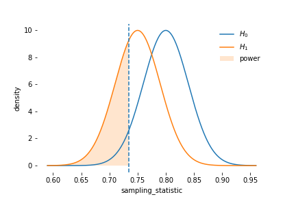
Example 1: Power of the Hypothesis Test of a Mean Score
This is a one-tailed t-test on population mean, but the sample size is large enough to treat it as a z test. You should verify that the numbers are correct.
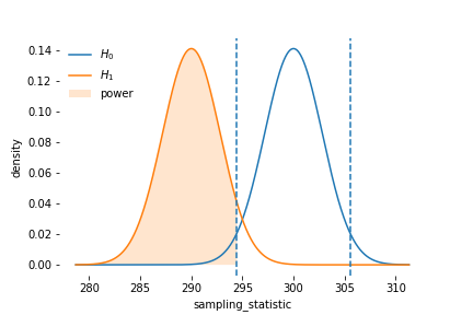
Example 2: Power of the Hypothesis Test of a Proportion
This is a two-tailed t-test on proportion, also solved as a z test. Notice here I did not truncate the probability at 100%.
Visualizing Power
Effect Size
Effect size is analogous to the size of the fish. Large fish are easier to catch. The animation shows that, as effect size increases, the empirical sampling distribution moves away from the one under the null.
Warning: do not interpret these two in a causal way. The sampling distribution does not move depending on how you change the effect size. In practice, we only get to observe the effect size after the experiment has ended, or guess about the effect size before the experiment starts. In either case, we have absolutely no control over the effect size.
Instead, understand the animation this way: when the center of the real sampling distribution is very far from that of the hypothesized one, it is easy to observe statistical significance between the two.
Alpha
Smaller alpha means we cannot afford to make Type I error. Conversely, as alpha increases (as shown in the animation), we become more tolerant of Type I error, and so we reject more often, if the null is true.
But when null is false, large alpha still allows us to reject more often, and so we acquire higher power.
Sample Size
This is guaranteed by the central limit theorem: standard error shrinks as the sample size grows. Visually, the sampling distribution becomes narrower and narrower (remember that standard error is simply the standard deviation of the sampling distribution).
Summary
This post should clarify some common logical fallacies regarding power. I hope you like the visualization. The animation code is available in my Kaggle notebook.
Extended Reading
The following blogs covers topics relevant to AB testing, and more in-depth review of key concepts mentioned in this article.


