Summary

The web content discusses the use of Poisson deviance as a loss function in regression models for count data, emphasizing its suitability over traditional mean squared error when dealing with over-dispersed or under-dispersed count data.

Abstract

The article delves into the Poisson distribution's application in regression models, particularly when the response variable represents count data such as the number of customers or events. It highlights the Generalized Poisson Models (GPMs) which accommodate variations in data dispersion. The piece explains the Poisson deviance, a loss function that is more appropriate for count data than the commonly used mean squared error (MSE) or root mean squared error (RMSE), as it does not penalize predictions that are above the mean as harshly, but significantly penalizes underestimations. This is particularly relevant when the mean of the Poisson distribution is high, and the data can be approximated by a Gaussian distribution. The author illustrates the Poisson deviance's behavior with graphical examples and contrasts it with other loss functions. The article also provides Python code snippets for calculating Poisson deviance and mentions the availability of Poisson loss functions in popular machine learning libraries.

Opinions

The author, Sachin Date, is recognized for providing clear explanations of complex topics, including Generalized Poisson Models (GPMs).
The mean squared error (MSE) is critiqued for its tendency to favor the median or mean, which may not be ideal for all datasets, especially those with count data.
The Poisson deviance is presented as a superior alternative to MSE for count data, as it better reflects the nature of the data by not excessively penalizing predictions that are slightly above the mean.
The author emphasizes the importance of using a loss function that aligns with the distribution of the data, noting that the Poisson distribution's log-likelihood function underpins the rationale for using Poisson deviance.
The article suggests that the Python libraries sklearn.metrics.mean_poisson_deviance and various Gradient Boosting libraries offer implementations of Poisson loss functions, facilitating their use in practical applications.
The author plans to explore the effectiveness of Poisson options in real-life datasets in future work, hinting at the practical value of this approach.

The Poisson Deviance for Regression

You’ve probably heard of the Poisson distribution, a probability distribution often used for modeling counts, that is, positive integer values. Imagine you’re modeling “events”, like the number of customers that walk into a store, or birds that land in a tree in a given hour. That’s what the Poisson is often used for. From the perspective of regression, we have this thing called Generalized Poisson Models (GPMs), where the response variable you are modeling is some kind of Poisson-ish type distribution. In a Poisson distribution, the mean is equal to the variance, but in real life, the variance is often greater (over-dispersed) or less than the mean (under-dispersed).

One of the most intuitive and easy to understand explanations of GPMs is from Sachin Date, who, if you don’t know, explains many difficult topics well. What I want to focus on here is something kind of related — the Poisson deviance, or the Poisson loss function.

Most of the time, your models, whether they are linear models, neural networks, or some tree-based method (XGBoost, Random Forest, etc.) are going to use mean squared error (MSE) or root mean squared error (RMSE) as your objective function. As you might know, MSE tends to favor the median, and RMSE and tends to favor the mean of a conditional distribution — this is why people worry about how the loss function works with the outliers in their data sets. However, most of the time, with some normally distributed response, you expect the values of the response (if z-score normalized, especially), to be some kind of Gaussian with mean 0 and unit variance. However, if you are dealing with count data — all positive integers — and you don’t scale or transform the response, then maybe a Poisson distribution is the better description of the data. When the mean of a Poisson is over 10, and especially over 20, it can be approximated with a Gaussian; the heavy tail that you see when the mean (the rate) is low tends to disappear.

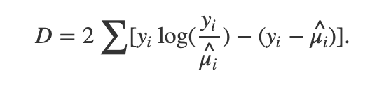
Take a look at the formula in the beginning of the post — the y_i is the ground truth, and the mu_i is your model’s prediction. Obviously, if y_i = mu_i, then you have a ln(1), which is 0, canceling out the first term, and the second as well, giving a deviance of 0. What’s interesting is what happens when your model errs on either side of the actual value. In the following snippet, I plot the loss of one example where the ground truth is set at 20 — meaning that we assume the variable is Poisson distributed with mean/rate = 20.

from matplotlib import pyplot as plt
import numpy as np

xticks = np.linspace(start = 0.0000, stop = 50, num = int(1e4))
yi = 20
losses = [2 * (yi * np.log(yi / x) - (yi - x)) for x in xticks]
losses = np.array(losses)
plt.scatter(xticks, losses)

Here’s the graph:

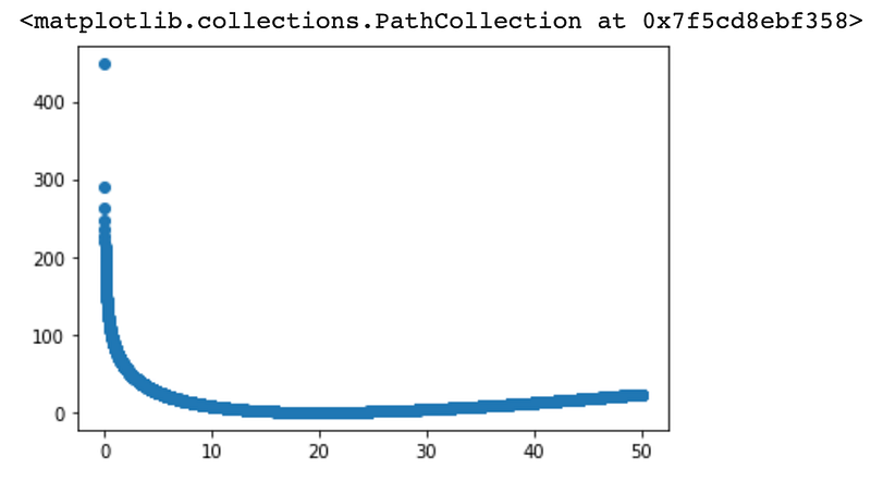
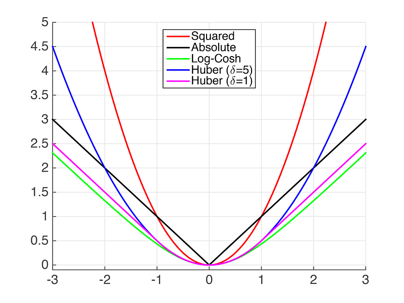
Poisson deviance as a function of model output. The rate/ground truth is set at 20 in this example, which is the minimum of the points you see here.

So what does this tell you? Well, if your model guesses between 10 and even 50, it doesn’t look like the deviance is that high — at least not compared with what happens if you guess 1 or 2. This is obviously a lot different from other loss functions:

So if your model outputs a 0 when the ground truth as 20, then, if you’re using MSE, the loss is 20² = 400, whereas, for the Poisson deviance, you would get infinite deviance, which is, uh, not good. The model isn’t supposed to really output 0, since there’s really not much probability mass there. If your model outputted something like .0001, your loss would be in the ballpark of >400. If your model outputs 30, and the ground truth was 20, your loss would only be around 3.78, where was in MSE terms, it would be 10² = 100.

So the moral of the story is that yes, the model should favor the mean of the distribution, but using Poisson deviance means you won’t penalize it that heavily for being biased ABOVE the mean — like if your model kept outputting 30 or 35, even if the distribution’s mean is 20. But your model will be penalized very heavily for outputting anything between 0 and 10. Why?

Well, what is the (log)likelihood function of the Poisson distribution?

Someone smarter than me did this:

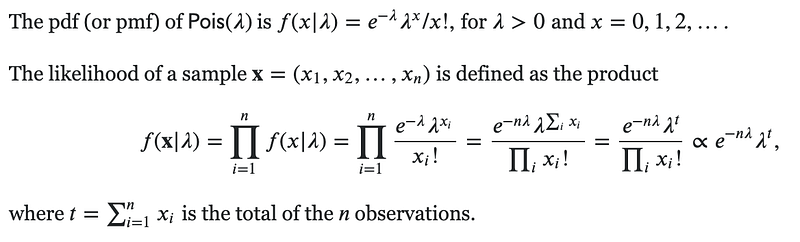
Now if you want to look at something a little more tractable, take the log of that —

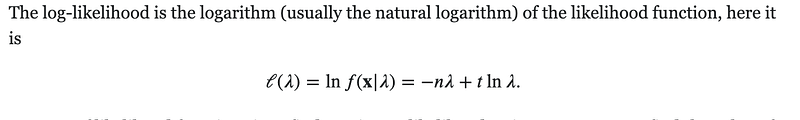
If your model keeps outputting 0, then t = 0, and that t * ln(lambda) expression is going to be 0, leaving you with a large negative number from the first term. In fact, the only way that your LL can even be close to “good” is if t — the sum of the observations — is sufficiently large for the second term to counteract the first term. That’s why, I believe, low values between 0–10 (again, assuming the rate/mean is 20) are penalized so heavily.

OK, so let’s say you’re sufficiently interested in the Poisson deviance. How can you calculate it? Well, from the perspective of the Python user, you have sklearn.metrics.mean_poisson_deviance — which is what I have been using. And you have Poisson loss as a choice of objective function for all the major GBDT methods — XGBoost, LightGBM, CatBoost, and HistGradientBoostingRegressor in sklearn. You also have PoissonRegressor() in the 0.24 release of sklearn…in any case, there are many ways you can incorporate Poisson type loss into training.

Does it help, though? Tune in for my next project, where I will see just how these Poisson options play out on real life data sets.