FAU Lecture Notes in Pattern Recognition

The Optimal Classifier

An introduction to the Bayes Classifier

These are the lecture notes for FAU’s YouTube Lecture “Pattern Recognition”. This is a full transcript of the lecture video & matching slides. The sources for the slides are available here. We hope, you enjoy this as much as the videos. This transcript was almost entirely machine generated using AutoBlog and only minor manual modifications were performed. If you spot mistakes, please let us know!

Navigation

Previous Chapter / Watch this Video / Next Chapter / Top Level

Welcome back, everybody to Pattern Recognition! So today we want to continue talking about the Bayesian Classifier, and today we want to introduce the optimality of the Bayesian Classifier.

So the Bayesian Classifier can now be summarized and constructed via the Bayesian decision rule. So, we essentially want to decide on the optimal class that is given here by y∗. y∗ is determined by the decision rule. Now what we want to do is we want to take the class that maximizes the probability given our observation x. We can express this with the base rule by constructing the actual prior for the class y. And then we need also the actual probability for the observation given class y, divided over the probability of observing the actual evidence. Now, since this is a maximization over y, we can actually get rid of the fraction here. And we can remove p(x) because it’s not changing the position of our maximum. So we can simply neglect it for the maximization. So this can then also be reformulated in the so-called log-likelihood function. And here we use the trick, that we apply the logarithm to this multiplication. This allows us to decompose the above multiplication into a sum of two logarithms. You will see that we will use this trick quite frequently in this class, so this is kind of an important observation. So you should definitely be aware of this and this will be very relevant for probably any kind of exam that you’re facing. So you should memorize this slide very well. Now this gives us the optimal decision according to the base rule. And there are some hints.

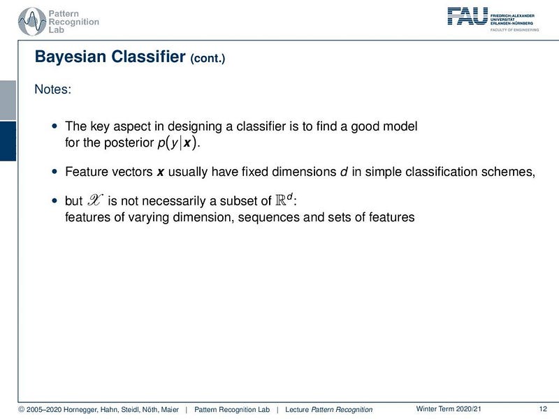
So typically, the key aspect for getting a good classifier is finding a good model for the posterior probability p of y given x. Then you typically have a fixed dimension in x. And this then gives rise to simple classification schemes. Then x is not necessarily a subset of the high dimensional space ℝᵈ, but it may be features of varying dimensions. For example, you observe that in sequences or sets of features. So for example, if you have a speech signal, then you don’t have a fixed dimension in d. But the same thing can be said faster or also slower. So this means then also that the number of observation changes. And this implies essentially a change in the dimensionality of your problem. So these are sequence problems where you then have to pick a kind of measure that will enable you to compare things of different dimensionality.

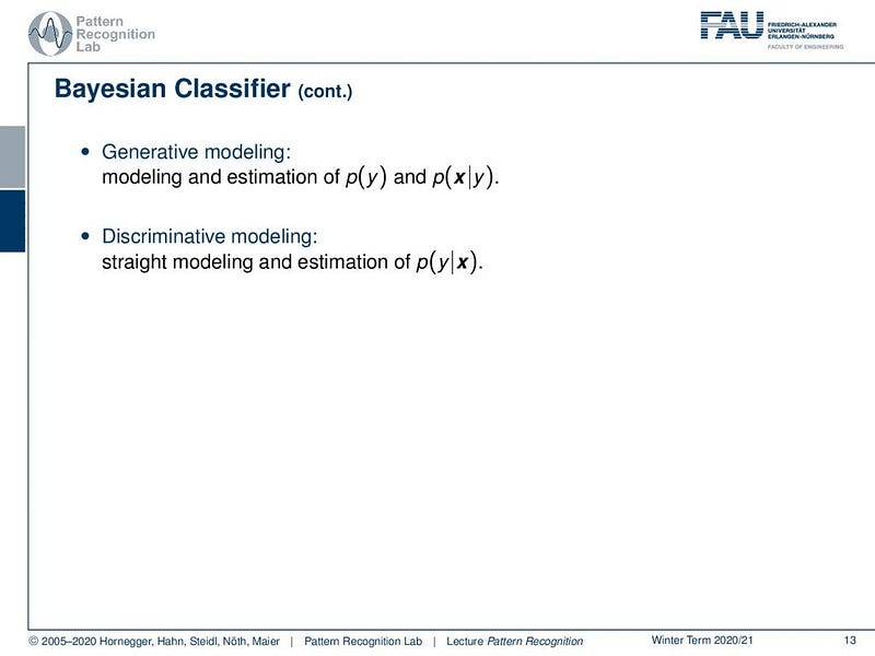
We typically analyze our problems either with generative modeling or with discriminative modeling. In generative modeling, you typically have a prior probability of the class y and then the distribution of your feature vectors x given the respective class. So here, you have a class conditional modeling, that is able to describe your entire feature space. And then you do the discriminative modeling in comparison. So here, you directly model the probability of the class, given the observations. This then enables us to find the decision very quickly. So essentially, we are modeling the decision boundary in this case.

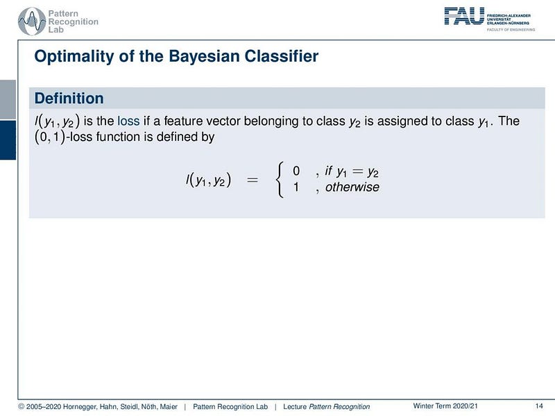
Let’s look a bit into the optimality of the Bayesian Classifier. If you attended Introduction to Pattern Recognition, you already have seen the formal proof that the Bayesian Classifier is the optimal classifier if you have a zero-one loss function and forced decision. Here, we only recall that you can associate any decision with a kind of risk or loss. This loss function then tells you what kind of damage is done if you decide for the wrong class. So essentially, the most frequently used example here is the zero-one loss function. And this essentially says you have a loss of one if you do a misclassification. It means that you treat all misclassifications equally and they have the same cost. And the correct classifications essentially have a cost of zero. So this is a very typical kind of loss function that is quite frequently used and in particular, people like to use it if they don’t know exactly what kind of cost is incurred by the misclassification. In these cases, you can then choose this kind of loss function. Now let’s see what happens if we use this loss function.

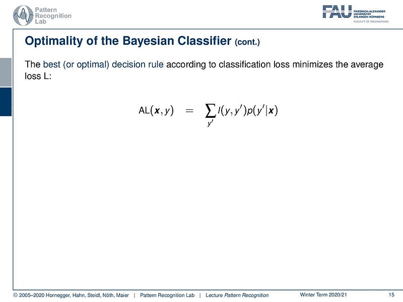
You can now argue with the minimization of the average loss and this is essentially what we want to do with the Bayesian Classifier. So we see we can write up the average loss as the expected value over the classes. Then we have the loss times the probability of the respective class given our observation. So this is now essentially the average loss for a given observation x. Now we want to decide on this observation.

This means that we want to minimize the average loss with respect to the classes. This is essentially a minimization of our average loss over the classes. So we can now plug in the original definition of our average loss. Now we seek to find the minimum given this loss. And now you can essentially see, because all of the misclassifications, which means the incorrect classes, will sum up to 1 minus the correct class probability. Then you can simply flip this minimization into the maximization of the probability of the correct class. So this is the reason why we find the solution for our optimal class as the maximization of the correct probability.

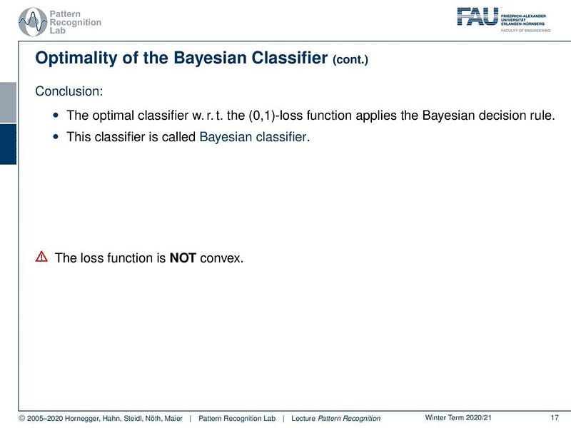
Now we can conclude that the optimal classifier concerning the zero-one loss function is actually generated by the Bayesian decision rule, and this classifier is called the Bayesian classifier. Note that this loss function is generally non-convex. So it sounds quite easy to do this maximization, but typically the real struggle is how to model the actual decision boundary. And essentially the main task that we will discuss in this class is that we look at different methods, in how to formulate these probabilities in order to determine the correct class.

So what are the lessons that we learned so far? We looked at the general structure of a classification system. We looked into supervised and unsupervised training, so we can also do training with only the observations without any labels. But of course, if we want to derive the class information, then we need labels. We looked into the basics of probabilities, probability, probability density function, the base rule, and so on. And we looked into the optimality of the base classifier and the role of the loss function. Also, we looked into the difference between discriminative and generative approaches to model the posterior probability.

So next time, we already want to look into the first classifiers, and we will start with the problem of logistic regression.

Of course, I can recommend a couple of further readings. The book by Niemann, which by the way also appeared in English, there is the book „Pattern Analysis“ and of course the german version „Klassifikation von Mustern“. Also, a very very good read is Duda and Hart’s book „Pattern Classification“.

So thank you very much for listening! I‘m looking forward to meeting you in the next video, bye-bye.

If you liked this post, you can find more essays here, more educational material on Machine Learning here, or have a look at our Deep Learning Lecture. I would also appreciate a follow on YouTube, Twitter, Facebook, or LinkedIn in case you want to be informed about more essays, videos, and research in the future. This article is released under the Creative Commons 4.0 Attribution License and can be reprinted and modified if referenced. If you are interested in generating transcripts from video lectures try AutoBlog.

References

Heinrich Niemann: Pattern Analysis, Springer Series in Information Sciences 4, Springer, Berlin, 1982.

Heinrich Niemann: Klassifikation von Mustern, Springer Verlag, Berlin, 1983.

Richard O. Duda, Peter E. Hart, David G. Stork: Pattern Classification, 2nd edition, John Wiley & Sons, New York, 2000.