
The Normal Distribution Simplified
Understanding one of the most important probability distributions and its application
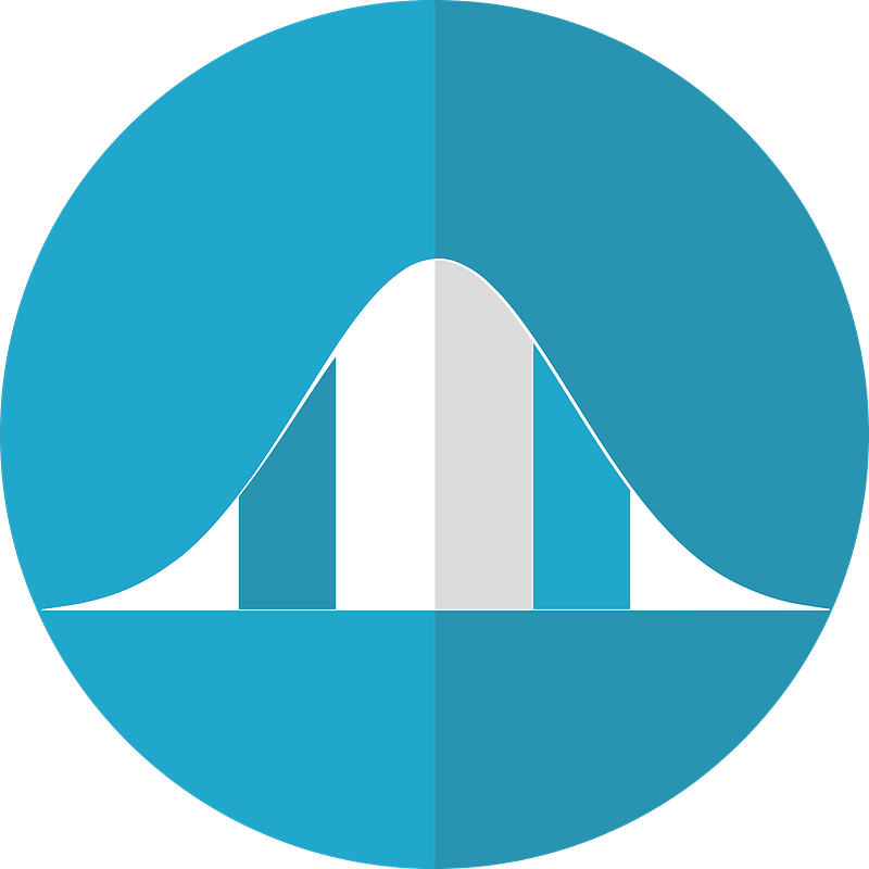
Even without being introduced to statistics, one may recognize the shape of the curve shown above. It is often perceived as a bell curve, but not many people actually know about its importance. The normal distribution is vital to the aspect of statistical inference, as it is often one of the conditions that even allow us to perform things like hypothesis tests. That is to say, if the probability distribution of a random variable is not normal, statistical inferences can not be made.
A normal probability distribution is symmetric around the mean, and the spread of the distribution is determined by the standard deviation of the data. Something special about this particular distribution is the 68–95–99.7 rule. The rule states that roughly 68%, 95%, and 99.7% of the data points are within one, two, and three standard deviations from the mean, respectively. This can be a useful shortcut to memorize the approximate way the data in a normal distribution is structured.
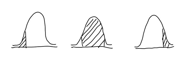
Now, this is all lovely and all, but do we ever observe data that is actually 100% normally distributed? Not really. So, there are a few conditions to check for normality, which, if satisfied, allow for the data to be granted the status of being approximately normally distributed. Here are two of the most practical ways to check for normality:
- Make a stem-leaf plot or a histogram out of the given data, and check if the shape resembles a normal distribution.
- Actually compute the percentage of values that fall within plus or minus one, two, and three standard deviations from the mean. If the values are around 68%, 95%, or 99.7%, respectively, you can assume that the data is approximately normally distributed.
Now that we’ve covered the basics of the normal distribution, let’s look at the usage of Z-Scores.
Z-Scores
The Z-Score is simply the number of standard deviations away from the mean. Note that this “number” can be either positive or negative, and it can either be a whole number or a decimal. A positive Z-Score means that that we are looking at data above the mean, while a negative Z-Score means that we are looking at data below the mean. When looking at a normal distribution, we can use Z-Scores to figure out the probability that a piece of data will fall below, within, or above certain standard deviation values.
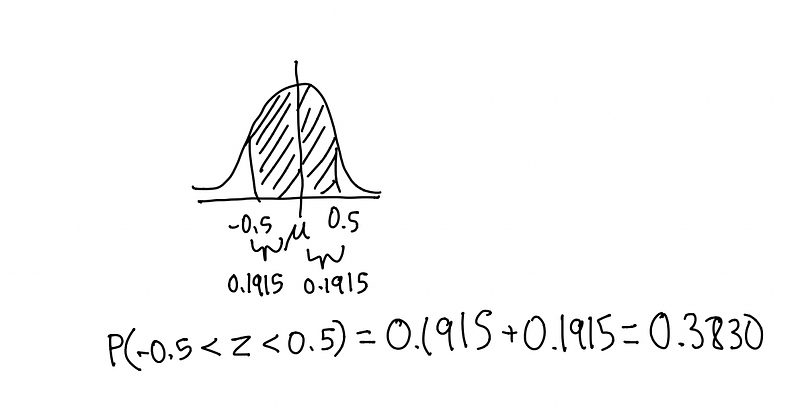
A typical problem may ask you to determine the percentage of values between 0.5 standard deviations from the mean. To solve this, we will need to use the Z-Score Table, which essentially tells us the probability that a value will fall within any number z standard deviations away from the mean. Going back to the original question, we are asked to find the value of P(-0.5 < z < 0.5). On our Z-Score Table, we see that z=0.5 gives us a probability of 0.1915. What’s cool here is that since the normal distribution is symmetric, the probabilities of P(-0.5 < z <0) and P(0 < z < 0.5) are both equal to the value of 0.1915 found earlier. The rest of the calculations come fluidly.
The fact that the normal distribution is symmetric is key in these kinds of problems. As mentioned before, the probabilities found in the Z-Score table will be the same for any positive and negative value of z (ex: -0.3 & 0.3, -1.2 & 1.2). Also, it will be nice to know that both P(z < 0) and P(z > 0) are 0.5, or 50%. Because of this, I encourage you to think about these probability questions in terms of area under the curve. For example, if you were asked to find the area between a square and its inscribed circle, you would subtract the area of the circle from the area of the square. Similarly, if you are asked to find the probability that a standard normal variable is greater than 0.55, you should subtract P(0 < z < 0.55) from 0.5. From there on out, it’s just a matter of finding the correct probability on the Z-Score table and making sure not to botch simple arithmetic.
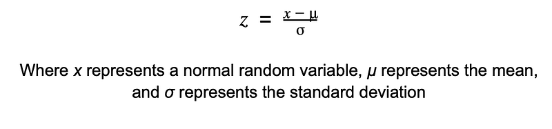
Z-Score Formula
In real world applications, it is not often that we are given the value of z. Sometimes, we need to find this value ourselves. To do this, we use the formula defined by the equation below.
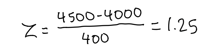
Let’s quickly look at an example. Suppose the weight of car at a certain company is normally distributed with mean 4,000 pounds and standard deviation 400 pounds. What is the probability of finding a car that is more than 4,500 pounds within the company?
Well, we first need to find our Z-Score using the formula provided.
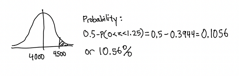
Afterwards, we can continue to solve for the probability.
Conclusion
The normal distribution is critical in the world of inferential statistics, and it encompasses many important parts of our world. For example, both height and IQ scores follow a normal distribution.