The Most Powerful Time Series Algorithm or How to Forecast Stocks in 2024

There are many algorithms that you can use to try to predict the returns of the stock market, but since the advent of deep learning, a particular type of recurrent neural network called LSTM (long short-term memmory) has been by far the most used for forecasting financial time series.

But not anymore. In this article, I am going to introduce the most modern and powerful algorithms used for stock forecasting in 2024 and will use the winner to forecast the monthly prices of the SP500 index.

As you probably know, the transformer, another type of neural network famous for powering large language models like ChatGPT has taken over the AI world, to the point that there is already a pretrained foundation model which relies on a transformer for time series forecasting called TimeGPT, it is in beta-version and you can subscribe to use its API here.

Basically, much like ChatGPT, TimeGPT is a transformer that has been pretrained with a huge amount of data (100 billion data points to be precise) of very different types of time series, allowing users to benefit from this huge computer power.

However, the transformer model is not the clear winner for time series problems as it is in the natural language type of problems, as you can see in the most important paper published on this topic recently, other models have achieved similar or even slightly better results in some cases:

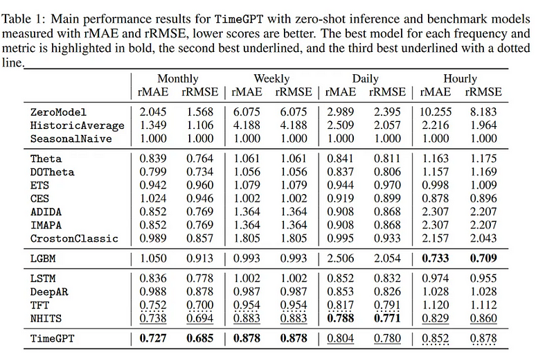
As you can see, the NHITS performs in a similar fashion as TimeGPT and even beats it with daily data, all in all, when you take into account its simplicity and the amount of easy-to-implement libraries available, then it emerges as a clear favorite in the current time series landscape.

The N-HITS algorithm is an extension of the N-BEATS, which is based on a stack of fully connected feedforward neural networks, where each network (called a “block”) is responsible for forecasting a specific horizon of the time series. The model consists of several such blocks stacked on top of each other, forming a multi-horizon forecasting system.

N-BEATS gained attention for its simplicity, scalability, and effectiveness in capturing temporal patterns in time series data. The model can handle both univariate and multivariate time series forecasting tasks.

However, the N-HITS is able to improve accuracy and reduce computational cost by incorporating hierarchical interpolation and sampling at different rates.

The idea of sampling time series at various rates to capture both short-term and long-term effects is an effective approach in time series forecasting. This allows the model to adapt to different temporal patterns and better capture the nuances of the data.

But don’t just believe my words about it, let’s get hands on and see how it works.

Predicting the Monthly Direction of the SP500 with NHITS

The data that I am using in this article has been compiled using a combination of the Fred Economic Data and the Quandl API . The FRED data offers a lot of financial data to download for free and the Quandl API comes in very handy to work with Python, once you create and account you can query lots of useful data easily, for example you can grab the pe ratio for SP500 like this:

!pip install quandl
dataset_code = "MULTPL/SP500_PE_RATIO_MONTH"
data = quandl.get(dataset_code)

My target variable is the price of the SP500 but what we actually want to predict is the monthly variation in stock prices of the SP500, basically we want to know if it will rise of fall (so we then buy or sell in consequence) therefore I have converted the target (prices of SP500) to a variable called “y_change” which measures how much the target changes from month to month.

Basing on this, if “y_change” is 0.05 it means stocks are up by 5%, and if it is -0.05 it means they are down 5% for that month. Also, I have included some exogenous variables which impact the stock prices, this will allow us to create a multivariable model for our time series which is interesting.

The data that I selected for this model includes:

• PE ratio: the most common metric to measure the value of stocks, when it is very high it means stocks are overvalued and viceversa
• FED interest rates: high interest rates are normally bad for the stock market and viceversa
• Consumer Price Index: growing inflation also has a negative impact on stock prices and viceversa
• Unemployment: also negative correlation with stocks

Taking this into account, this is how my historical dataframe with data from 1955 until present looks like:

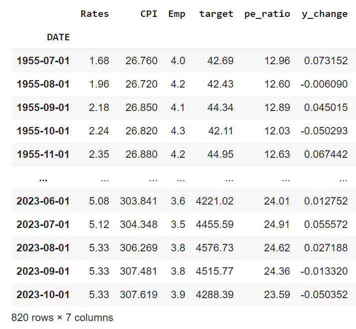
Great, now let’s see how to use the darts library to train our N-HITS model and try to predict if stocks are going up or down next month.

When you look at the code below you will realize that this library has really succeeded at taking out complexity and lets you code your models in a super simple way:

from darts import TimeSeries
from darts.models import NHiTSModel
from darts.dataprocessing.transformers import Scaler

#loading data into a Darts TimeSeries object
#covariates are the columns with the variables we believe will influence our target
#target in this case is the y_change column with the monthly change in SP500 pricess
covariates = TimeSeries.from_dataframe(df, time_col='date_time', value_cols=['Rates', 'CPI', 'Emp', 'pe_ratio'])
target = TimeSeries.from_dataframe(df, time_col='date_time', value_cols=['y_change'])

#the time window is 24 so 2 years in this case and will try to predict 12 months ahead
past = 24
future = 12

#always scale the data
cov_scaler = Scaler()
target_scaler = Scaler()
scaled_target = target_scaler.fit_transform(target)
scaled_covariates = cov_scaler.fit_transform(covariates)

#splitting data into train (80% of data) and test sets (20% of data)
y_train, y_test = target[:655], target[655:]
X_train, X_test = covariates[:655], covariates[655-past:]

#initialize and train the NHiTSModel
model = NHiTSModel(input_chunk_length=past, output_chunk_length=future,n_epochs=50)

#fit the model with target and past covariates
model.fit(y_train, past_covariates=X_train)

#forecasting future n months (164 months in this case) using the trained model
prediction = model.predict(n=164,past_covariates=X_test)

#plot predictions vs real values
y_test.plot('Real Values')
prediction.plot(label='N-HiTS')

Now, this is the graph we get from the plotting we have done:

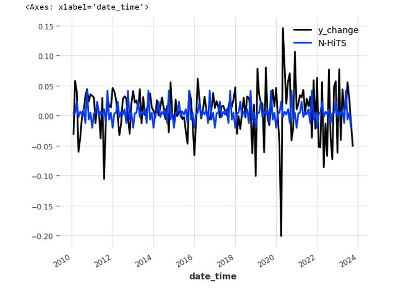
As we can see, we didn’t do any for loop, the dart library has done it under de hood for us, it has iterated over 164 months (more than 13 years) and it has looked at the previous 24 months in order to predict the next 12 months, moving the window accordingly for us, I believe for a quant this is pretty cool stuff, to have such a high level library available.

OK, cool, so now how good were these predictions?

Well, we need to see how many monthly changes have the same sign in the test dataset versus our predictions, we can do it like this:

#create a dataframe with results
results = pd.DataFrame(y_test[1:].pd_series().values, columns=['Real'])
results['Preds'] = prediction.pd_series().values

#calculate the summation of cases where prediction and test have same sign
sum(results['Preds']*results['Real']>0)

In this case, I got 96 matches

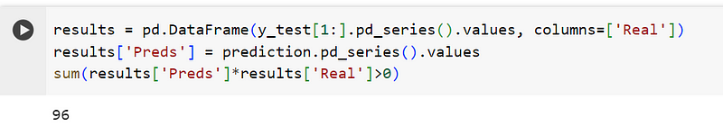
So, 96 times out of 164 months means we were right 58.54% of the time, how does it sound to you? Is it good or bad?

Well, let’s try to understand the results and see if we can learn from them.

Analyzing Results

If we want to measure how good these results are, the first thing we need to do is to compare how they perform against the simplest strategy which is just buying and holding.

For the period of time in our test set we had 108 positive days, so just being long all the time would have been better than following the predictions of our model, however, this was a very bullyish period of time in history.

If we look at the full dataset we will discover that from 1955 until 2023 there were 500 positive months and 320 negative ones, which means that historically, the probability of a positive return for a given month is about 60% which is more or less what we achieved at 58.54%.

Yes, we could keep fine tuning our model but I am pretty sure we won’t achieve a significantly higher result, and this takes me to the most important point in this article: no matter how good and modern your time series algorithm is, time series forecasting is not well suited for predicting stock prices.

The Problem with Time Series and Stock Forecasting

When you try to predict the direction of stock prices, there is a “main direction” called draft, which goes up, because stocks always go up given enough time. Then there are also periodic oscillations, and if we could predict them, we would make money every month, because we would make money when they go up and also when they go down.

But the problem is that these periodic oscillations don’t follow a seasonal pattern, stock prices are not a physical variable that obey a general rule, instead, their variance is affected by countless variables which on top of that also change constantly, therefore the variance of stocks follows a random pattern.

In other words, you know there will be around 60% positive months alternated by 40% negative months, but you don’t know when they will happen.

The problem is not that time series or deep learning doesn’t work, they both actually work very powerfully, the problem is we are using the wrong kind of tool for the wrong kind of problem. There are problems like predicting daily temperatures or daily energy demands that indeed are suited for time series algorithms, but sequences of stock prices do not repeat themselves periodically.

Does this mean you cannot make money in stocks as a quant? Of course not, quants make huge amounts in stocks, but they don’t do it using time series forecasting.

What Really does Work for Stock Forecasting

So, if time series don’t work, then what do successful quants do?

Well, to think as a quant, the first thing you need to do is to start thinking in probabilities, that means thinking with a Bayesian Mindset. This is a change of paradigm because you don’t focus on predictions, you focus on measuring how good are your predictions, and managing risk in consequence, that is where the skills of a trader really shine.

Instead of getting caught up trying to use the most powerful deep learning algorithm to perfectly predict every move of stock prices, you need to realize that the money is not in perfect predictions.

Betting in the stock market is like any other type of betting, you don’t need to be sure of something to make money, actually as the famous Nasim Taleb has pointed out many times, you can make a lot of money by realizing that other people are very sure of things when in fact they cannot predict them.

If you want to see how to start applying Bayesian Networks to the stock market you can read my previous article in which I introduce the concepts of bayesian thinking and then I code an example in Python.

Also if you enjoyed this, don’t forget to click the subscribe button because in my future articles I will talk in depth about how to use quantitative strategies, artificial intelligence and probabilistic methods.