The Modified Fisher RSI. A Powerful Contrarian Technical Indicator.

Combining the RSI with the Modified Fisher Transform to Trade the Market.

Structured indicators are created by fusing two or more other indicators. These transformations are very useful and open new horizons with regards to trading optimization and signals. In this article, we will combine the famous relative strength index with the Fisher transform to create the Fisher strength index which is a powerful contrarian indicator. We will first introduce the two indicators before seeing how to combine them.

I have just released a new book after the success of my previous one “The Book of Trading Strategies”. It features advanced trend-following indicators and strategies with a GitHub page dedicated to the continuously updated code. Also, this book features the original colors after having optimized for printing costs. If you feel that this interests you, feel free to visit the below Amazon link, or if you prefer to buy the PDF version, you could contact me on LinkedIn.

The Relative Strength Index

The RSI is without a doubt the most famous momentum indicator out there, and this is to be expected as it has many strengths especially in ranging markets. It is also bounded between 0 and 100 which makes it easier to interpret. Also, the fact that it is famous, contributes to its potential.

This is because the more traders and portfolio managers look at the RSI, the more people will react based on its signals and this in turn can push market prices. Of course, we cannot prove this idea, but it is intuitive as one of the basis of Technical Analysis is that it is self-fulfilling.

The RSI is calculated using a rather simple way. We first start by taking price differences of one period. This means that we have to subtract every closing price from the one before it. Then, we will calculate the smoothed average of the positive differences and divide it by the smoothed average of the negative differences. The last calculation gives us the Relative Strength which is then used in the RSI formula to be transformed into a measure between 0 and 100.

To calculate the relative strength index, we need an OHLC array (not a data frame). This means that we will be looking at an array of 4 columns. The function for the Relative Strength Index is therefore:

# The function to add a number of columns inside an array
def adder(Data, times):
    
    for i in range(1, times + 1):
    
        new_col = np.zeros((len(Data), 1), dtype = float)
        Data = np.append(Data, new_col, axis = 1)
        
    return Data

# The function to delete a number of columns starting from an index
def deleter(Data, index, times):
    
    for i in range(1, times + 1):
    
        Data = np.delete(Data, index, axis = 1)
        
    return Data
    
# The function to delete a number of rows from the beginning
def jump(Data, jump):
    
    Data = Data[jump:, ]
    
    return Data

# Example of adding 3 empty columns to an array
my_ohlc_array = adder(my_ohlc_array, 3)

# Example of deleting the 2 columns after the column indexed at 3
my_ohlc_array = deleter(my_ohlc_array, 3, 2)

# Example of deleting the first 20 rows
my_ohlc_array = jump(my_ohlc_array, 20)

# Remember, OHLC is an abbreviation of Open, High, Low, and Close and it refers to the standard historical data file

def ma(Data, lookback, close, where): 
    
    Data = adder(Data, 1)
    
    for i in range(len(Data)):
           
            try:
                Data[i, where] = (Data[i - lookback + 1:i + 1, close].mean())
            
            except IndexError:
                pass
            
    # Cleaning
    Data = jump(Data, lookback)
    
    return Datadef ema(Data, alpha, lookback, what, where):
    
    alpha = alpha / (lookback + 1.0)
    beta  = 1 - alpha
    
    # First value is a simple SMA
    Data = ma(Data, lookback, what, where)
    
    # Calculating first EMA
    Data[lookback + 1, where] = (Data[lookback + 1, what] * alpha) + (Data[lookback, where] * beta)    
 
    # Calculating the rest of EMA
    for i in range(lookback + 2, len(Data)):
            try:
                Data[i, where] = (Data[i, what] * alpha) + (Data[i - 1, where] * beta)
        
            except IndexError:
                pass
            
    return Data

def rsi(Data, lookback, close, where):
    
    # Adding a few columns
    Data = adder(Data, 5)
    
    # Calculating Differences
    for i in range(len(Data)):
        
        Data[i, where] = Data[i, close] - Data[i - 1, close]
     
    # Calculating the Up and Down absolute values
    for i in range(len(Data)):
        
        if Data[i, where] > 0:
            
            Data[i, where + 1] = Data[i, where]
            
        elif Data[i, where] < 0:
            
            Data[i, where + 2] = abs(Data[i, where])
            
    # Calculating the Smoothed Moving Average on Up and Down absolute values    
    lookback = (lookback * 2) - 1 # From exponential to smoothed
    Data = ema(Data, 2, lookback, where + 1, where + 3)
    Data = ema(Data, 2, lookback, where + 2, where + 4)    

    # Calculating the Relative Strength
    Data[:, where + 5] = Data[:, where + 3] / Data[:, where + 4]
    
    # Calculate the Relative Strength Index
    Data[:, where + 6] = (100 - (100 / (1 + Data[:, where + 5])))   

    # Cleaning
    Data = deleter(Data, where, 6)
    Data = jump(Data, lookback)    

    return Data

If you want to see more articles, consider subscribing to my DAILY Newsletter (A Free Plan is Available) via the below link. It features my Medium articles, more trading strategies, coding lessons related to research and analysis, also, subscribers get a free PDF copy of my first book. You can expect 5–7 articles per week with your paid subscription and 1–2 articles per week with the free plan. This would help me continue sharing my research. Thank you!

The Fisher Transform

One of the pillars of descriptive statistics is the normal distribution curve. It describes how random variables are distributed and centered around a central value. It often resembles a bell. Some data in the world are said to be normally distributed.

This means that their distribution is symmetrical with 50% of the data lying to the left of the mean and 50% of the data lying to the right of the mean. Its mean, median, and mode are also equal as seen in the below curve.

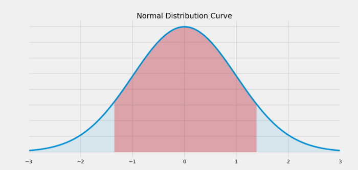
The above curve shows the number of values within a number of standard deviations. For example, the area shaded in red represents around 1.33x of standard deviations away from the mean of zero. We know that if data is normally distributed then:

• About 68% of the data falls within 1 standard deviation of the mean.
• About 95% of the data falls within 2 standard deviations of the mean.
• About 99% of the data falls within 3 standard deviations of the mean.

Presumably, this can be used to approximate the way to use financial returns data, but studies show that financial data is not normally distributed. For the moment, we can assume it is so that we can use such indicators. The flaw of the method does not hinder much its usefulness.

Let us now see how to create the modified Fisher transformation which is basically like the original one but with some minor changes to enhance the results and make them easier to obtain.

Created John F. Ehlers, the indicator seeks to transform the price into a normal Gaussian (normal) distribution. This is very helpful in detecting reversals which is the main point of the article. The steps to create the modified Fisher transform are somewhat similar to the original Fisher transform. Here is how we do it:

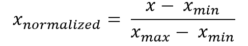
• Select a lookback period and calculate a normalized version of the OHLC data using the formula as seen below:

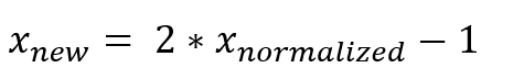
• Trap the values from the first step between -1 and +1 using the following normalization formula:

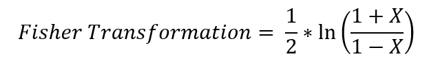
• Create a condition that eliminates the -1.00’s and +1.00’s and transforms them into -0.999’s and +0.999’s so that we do not get infinite values. This also serves to make the indicator bounded between two levels we will see later.
• Apply the following formula to the results from the last step:

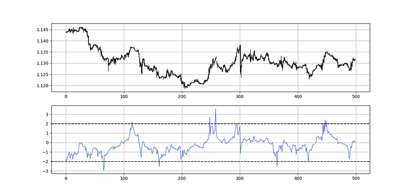
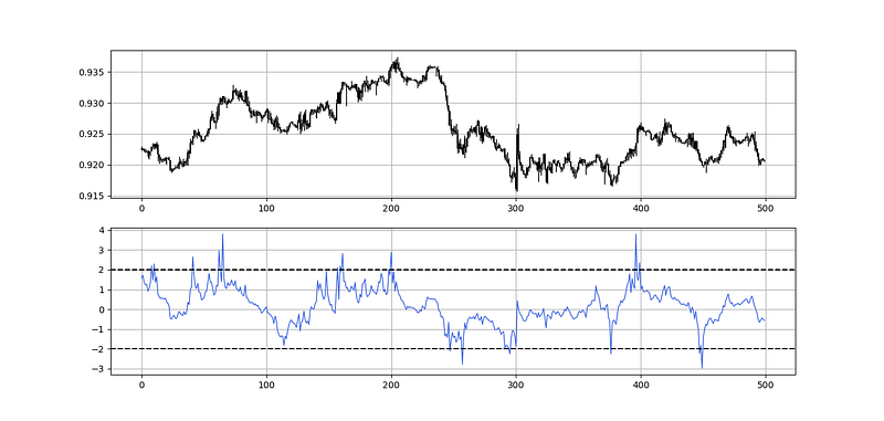
Now that we have the modified Fisher transformation indicator, we can proceed by coding it in Python. The below plot shows a 5-period modified Fisher transformation with boundaries at -2.00 and +2.00.

def stochastic_oscillator(data, 
                             lookback, 
                             high, 
                             low, 
                             close, 
                             where, 
                             slowing = False, 
                             smoothing = False, 
                             slowing_period = 1, 
                             smoothing_period = 1):
            
    data = adder(data, 1)
        
    for i in range(len(data)):
            
        try:
            
            data[i, where] = (data[i, close] - min(data[i - lookback + 1:i + 1, low])) / (max(data[i - lookback + 1:i + 1, high]) - min(data[i - lookback + 1:i + 1, low]))
            
        except ValueError:
            
            pass
        
    data[:, where] = data[:, where] * 100  
            
    if slowing == True and smoothing == False:
        
        data = ma(data, slowing_period, where, where + 1)
    
    if smoothing == True and slowing == False:
        
        data = ma(data, smoothing_period, where, where + 1)
        
    if smoothing == True and slowing == True:
    
        data = ma(data, slowing_period, where,   where + 1)
        
        data = ma(data, smoothing_period, where, where + 2)        
       
    data = jump(data, lookback)

    return data

def fisher_transform(data, lookback, high, low, close, where):
    
   data = adder(data, 1)
   
   data = stochastic_oscillator(data, lookback,  high, low, close, where)
   
   data[:, where] = data[:, where] / 100
   
   data[:, where] = (2 * data[:, where]) - 1
   
   for i in range(len(data)):
       
       if data[i, where] == 1:
           
           data[i, where] = 0.999
           
       if data[i, where] == -1:
           
           data[i, where] = -0.999
           
   for i in range(len(data)):
       
      data[i, where + 1] = 0.5 * (np.log((1 + data[i, where]) / (1 - data[i, where])))
   
   data = deleter(data, where, 1)   
   
   return data

Naturally with the correction I have added, the maximum values will be 3.80 and the minimum values will be -3.80. Therefore, we can say that the indicator is now bounded even though the original version was not shown to be bounded.

If you are also interested by more technical indicators and strategies, then my book might interest you:

The Fisher Strength Index

This indicator which we can call the Fisher strength index is nothing but the application of the relative strength index function to the Fisher transform values which have been applied to the market price.

To simple code this, we can use the following code:

lookback_rsi =  14
lookback_fisher = 55

my_data = fisher_transform(my_data, lookback_fisher, 1, 2, 3, 4)
my_data = rsi(my_data, lookback_rsi, 4, 5)

Which should give us plots like the following. The default barriers I have found to be optimal for a 14-period Fisher Strength Index are 75 and 25.

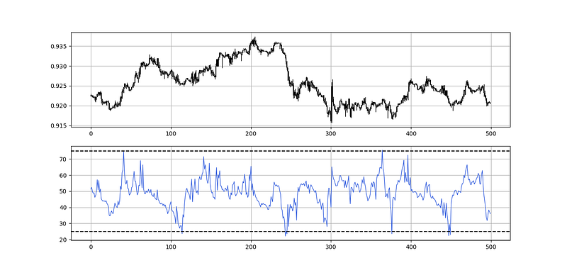
Note that the indicator can also be used in discretionary trading and while the default parameters are 55 for the Fisher Transform and 14 for the RSI, you can modify and optimize them as you wish.

Conclusion

Remember to always do your back-tests. You should always believe that other people are wrong. My indicators and style of trading may work for me but maybe not for you.

I am a firm believer of not spoon-feeding. I have learnt by doing and not by copying. You should get the idea, the function, the intuition, the conditions of the strategy, and then elaborate (an even better) one yourself so that you back-test and improve it before deciding to take it live or to eliminate it. My choice of not providing specific Back-testing results should lead the reader to explore more herself the strategy and work on it more.

Medium is a hub to many interesting reads. I read a lot of articles before I decided to start writing. Consider joining Medium using my referral link!

To sum up, are the strategies I provide realistic? Yes, but only by optimizing the environment (robust algorithm, low costs, honest broker, proper risk management, and order management). Are the strategies provided only for the sole use of trading? No, it is to stimulate brainstorming and getting more trading ideas as we are all sick of hearing about an oversold RSI as a reason to go short or a resistance being surpassed as a reason to go long. I am trying to introduce a new field called Objective Technical Analysis where we use hard data to judge our techniques rather than rely on outdated classical methods.