The lad’s guide to R

R is a programming language and free software environment which is popular in the mathematics and statistics community. As the field of Data Science grows and starts to popularize it should start gaining more importance for it’s a great simple tool to handle Big Data, which all tech companies know is where the next bounty to compete for will be. In this guide, we’ll review multiple applications which use R so that anyone can use it as a reference guide and introduction to how this powerful tool works.

Computing Probabilities with R

> p.supplier <- c(0.089392188, 0.128777308, 0.039405122, 0.020865516, 0.035332313, 0.578176022 ,
+ 0.002072526, 0.011297042, 0.058540258, 0.036141705)
> p.supplier.defective <- c(0.0187877518, 0.0005842148, 0.0140875989, 0.0044491375,
+ 0.0082523774 , 0.0036521773, 0.0033200327, 0.0100657919, 0.0136377822, 0.0054586565)
> p.defective <- p.supplier.defective %*% p.supplier
> p.supplier[1]*p.supplier.defective[1]/p.defective
 [,1]
[1,] 0.2835958

The probability that supplier a produced the defective fastener given that it was defective is 0.2835958

> p <- vector(length = 10) 
> for (i in 1:10) p[i] <- p.supplier[i] * p.supplier.defective[i] / p.defective
> p
 [1] 0.283595775 0.012703906 0.093737859 0.015675822 0.049235293 0.356563845
 [7] 0.001161897 0.019201629 0.134810512 0.033313463

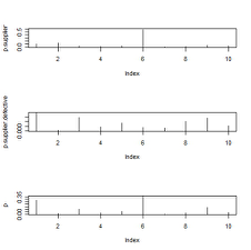
Supplier six is the most likely to be producing defective fastener units. This answer was found with probability, and can also be seen in the plots later on. Nevertheless, supplier six is also the one which provides the most groups, so it is logical that it also presents the most defective units as seen in the computed probability.

> par(mfrow=c(3, 1))
> plot(p.supplier, type=”h”)
> plot(p.supplier.defective, type=”h”)
> plot(p, type=”h”)
> ?plot
> par(mfrow=c(3, 1))
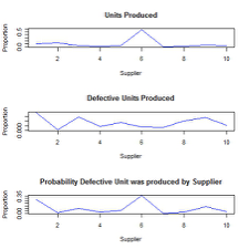
> plot(p.supplier, type=”l”, main=”Units Produced”, xlab=”Supplier”, ylab=”Proportion”, col=”blue”)
> plot(p.supplier.defective, type=”l”, main=”Defective Units Produced”, xlab=”Supplier”, ylab=”Proportion”, col=”blue”)
> plot(p, type=”l”, main=”Probability Defective Unit was produced by Supplier”, xlab=”Supplier”, ylab=”Proportion”, col=”blue”)

It is evident in both the histogram plot and line plot that the supplier that is the most likely to produce a defective unit is supplier six.

Computing Number of Potential Outcomes with R

> choose(100,5)
[1] 75287520

Out of a population of size one hundred, there are 75287520 ways of getting a size sample of size five.

> choose(95,5)
[1] 57940519
> choose(5,100)
[1] 0
> choose(95,5)*choose(5,0)
[1] 57940519
> choose(95,5)/choose(100,5)
[1] 0.76959

Out of a population of size ninety-five, there are 57940519 ways of getting a size sample of size five.

Out of a population of size five, there is 1 way of getting a size sample of size five.

The proportion of the samples that do not include handicapped students is 0.76959, so to take this minority into account, one should target them.

Computing the Probability Mass Function of a File with R

> load(“V:\\Downloads\\P.RData”)
> length(which(p1<0))
[1] 0
> sum(p1)
[1] 1
> length(which(p2<0))
[1] 0
> sum(p2)
[1] 0.81
> length(which(p3<0))
[1] 58
> sum(p3)
[1] 1

P1 is the PMF of a random variable because its values all sum to 1 and are all in between zero and 1.

P2 cannot be the PMF of a random variable because its values do not sum to 1 even though they are all in between zero and 1.

P3 cannot be the PMF of a random variable because some of its values are less than zero, even though they all sum to 1.

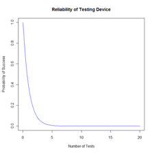
Finding Discrete Random Variables with R

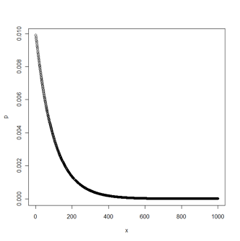
> x=c(1:1000)
> p=dgeom(x,prob=.01)
> plot(x,p)
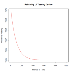
> plot(x,p, type=”l”, col=”red”, main=”Reliability of Testing Device”, xlab=”Number of Tests”, ylab=”Probability Passing”)
> rgeom(5,0.009)
[1] 222 161 51 429 133

X is a discrete random variable because it is countable even when infinite.

Pass = θ^n Fail = (θ-1) P(x) = θx(1- θ)

Using the Geometric distribution for 5 observations with a probability of success in each trial with the likelihood of success for 0.009 we would get the 5 following random deviates: 222, 161, 51, 429, 133.

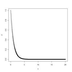
Computing the Probability Density Function with R

> dexp(0.01, rate=100, log=FALSE) 
[1] 36.78794
> x=seq(0,20,length=1000)
> p=dexp(x,rate=1)
> plot(x,p)
> plot(x,p, type=”l”, col=”blue”, main=”Reliability of Testing Device”, xlab=”Number of Tests”, ylab=”Probability of Success”)
> rexp(1, rate = 1)
[1] 0.9120144

It equals 36.78794 which is greater than 1, and this is because it only is a density function, not necessarily the probability per se.

If one test with theta equal one were taken out of the exponential distribution of the PDF, then we would get a random deviate value of 0.9120144.

Computing Likelihood Function with R

> logl <- function(n, y, theta)
+ {
+ n * log(theta) — theta * y
+ }
> set.seed(2012)
> x <- rexp(n=1e+2, rate=2)
> y <- sum(x)
> logl(n=1e+2, y=y, theta=2)
[1] -44.01345

The R function logl is an algorithmic representation in the code of the function l(θ). In the code representation of the function, n represents the sample size, theta represents the probability of the function and y is each value of the variable in the sample space, like xi in mathematical notation.

> curve(logl(n=1e+2, y=y, theta=x), xlim=c(0,20))
> mle.theta <- 1e+2/y
> mle.theta
[1] 1.764786
> abline(v=mle.theta, col=”red”)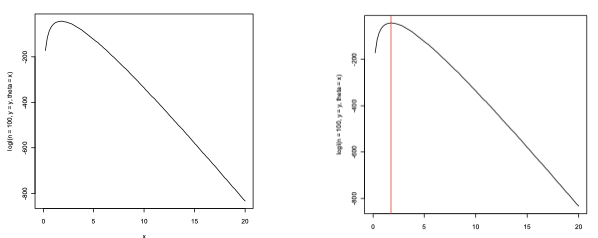

Computing Maximum Likelihood Estimation with R

> x <- rexp(n=1e+7, rate=2)
> mle.theta <- vector(length = 7)
> mle.theta[1] <- 1e+1/sum(x[1:1e+1])
> mle.theta[2] <- 1e+2/sum(x[1:1e+2])
> mle.theta[3] <- 1e+3/sum(x[1:1e+3])
> mle.theta[4] <- 1e+4/sum(x[1:1e+4])
> mle.theta[5] <- 1e+5/sum(x[1:1e+5])
> mle.theta[6] <- 1e+6/sum(x[1:1e+6])
> mle.theta[7] <- 1e+7/sum(x[1:1e+7])
> plot(x=c(1:7), mle.theta, ylim=c(0,4), type=”l”)
> abline(h=2, col=”red”)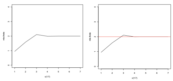

Because the sample size is the numerator of the function, it is expected that the function will continuously increase until reaching its peak at the value of the MLE, which goes accordingly to our previous results. Then as the size of the sample approaches infinity, the amount of the estimator theta-hat will also approximate the real value of theta; hence that is why it’s called an estimator.

Finding an External Data’s Regression Line with R

> x <- read.table("data.dat")

> x

V1 V2 V3 V4 V5

1   1 80 27 89 42

2   2 80 27 88 37

3   3 75 25 90 37

4   4 62 24 87 28

5   5 62 22 87 18

6   6 62 23 87 18

7   7 62 24 93 19

8   8 62 24 93 20

9   9 58 23 87 15

10 10 58 18 80 14

11 11 58 18 89 14

12 12 58 17 88 13

13 13 58 18 82 11

14 14 58 19 93 12

15 15 50 18 89  8

16 16 50 18 86  7

17 17 50 19 72  8

18 18 50 19 79  8

19 19 50 20 80  9

20 20 56 20 82 15

21 21 70 20 91 15

> line <- lm(x[,5] ~ x[,3])

> summary(line)

Call:

lm(formula = x[, 5] ~ x[, 3])

Residuals:

Min      1Q  Median      3Q     Max

-7.8904 -3.6206  0.3794  2.8398  8.4747

Coefficients:

Estimate Std. Error t value Pr(>|t|)

(Intercept) -41.9109     7.6056  -5.511 2.58e-05 ***

x[, 3]        2.8174     0.3567   7.898 2.03e-07 ***

---

Signif. codes:  0 ‘***’ 0.001 ‘**’ 0.01 ‘*’ 0.05 ‘.’ 0.1 ‘ ’ 1

Residual standard error: 5.043 on 19 degrees of freedom

Multiple R-squared: 0.7665,     Adjusted R-squared: 0.7542

F-statistic: 62.37 on 1 and 19 DF,  p-value: 2.028e-07

> plot(x[,3], x[,5])

> abline(reg=line)

V1 V2 V3 V4 V5

1   1 80 27 89 42

2   2 80 27 88 37

3   3 75 25 90 37

4   4 62 24 87 28

5   5 62 22 87 18

6   6 62 23 87 18

7   7 62 24 93 19

8   8 62 24 93 20

9   9 58 23 87 15

10 10 58 18 80 14

11 11 58 18 89 14

12 12 58 17 88 13

13 13 58 18 82 11

14 14 58 19 93 12

15 15 50 18 89  8

16 16 50 18 86  7

17 17 50 19 72  8

18 18 50 19 79  8

19 19 50 20 80  9

20 20 56 20 82 15

21 21 70 20 91 15

Call:

lm(formula = x[, 5] ~ x[, 3])

Residuals:

Min      1Q  Median      3Q     Max

-7.8904 -3.6206  0.3794  2.8398  8.4747

Coefficients:

Estimate Std. Error t value Pr(>|t|)

(Intercept) -41.9109     7.6056  -5.511 2.58e-05 ***

x[, 3]        2.8174     0.3567   7.898 2.03e-07 ***

---

Signif. codes:  0 ‘***’ 0.001 ‘**’ 0.01 ‘*’ 0.05 ‘.’ 0.1 ‘ ’ 1

Residual standard error: 5.043 on 19 degrees of freedom

Multiple R-squared: 0.7665,     Adjusted R-squared: 0.7542

F-statistic: 62.37 on 1 and 19 DF,  p-value: 2.028e-07

The line summary displays the characteristics of the regression line in comparison to data, given the range and an established hypothesis with our regression formula.

In the table, we can read almost all of the statistical summaries for the regression line. From this data, we can interpret that given the small p-value we can reject the fact that the slope of the regression line is zero, giving the result seen above with a line and a slope showing the actual relationship between the data and the regression.

Given the multiple R-squared, we can see that the variance of the new relationship given the regression line with a slope is actually quite good. Also given the new regression line relationship we could determine the correlation given the data by viewing the F-statistic value.

Finding the Exponential Distribution of a DataSet with R

> y<-rexp(50,rate=0.5)

> y

[1] 0.76119331 2.96264641 5.29070748 1.06243433 7.93300776 0.31884968

[7] 1.36268596 4.58369499 0.42588764 3.29949299 0.26702438 2.07610880

[13] 2.31741453 1.61899089 1.57655291 1.16621485 0.54150387 3.56295922

[19] 2.94792584 5.68264995 5.26944757 3.34124570 4.43604455 6.02521655

[25] 2.12544993 2.33883546 4.35960364 2.13570019 4.27275216 3.67030518

[31] 0.63136411 4.57124798 0.93281055 1.04153006 2.40677084 1.92769461

[37] 1.52501945 1.16928538 0.03694785 0.31678147 0.85142687 2.91888848

[43] 2.70040629 2.95351881 3.03363597 0.99829758 7.74753467 2.29434603

[49] 0.45836493 1.74184175

> p<-pexp(rate=0.5, q=1)

> p

[1] 0.3934693

> s<-length(which(y<1))

> s

[1] 12

> pbinom(s, 50, p)

[1] 0.01672091

Finding the Mean and Variance of a DataSet with R

> set.seed(12502579)

> sample.means.1 <- vector(length=10000)

> for (i in 1:10000)

+ {

+ sample.means.1[i] <- sum(rexp(rate=.5,n=50))/50

+ }

> sample.means.1

> mean(sample.means.1)

[1] 2.000342

> expmean<-1/(rate=0.5)

> expmean

[1] 2

The expectation of the mean was very close to the mean of the sample means because the expected value is a weighted average, hence almost a mean itself.

> var(sample.means.1)

[1] 0.08061066

> expvar<-1/(rate=0.5)^2

> samplevar<-expvar/50

> samplevar

[1] 0.08

The expected variance was very close to the variance of the sample mean because both have exponential distribution so the spread of the values is similar.

> set.seed(12502579)

> sample.means.2 <- vector(length=10000)

> for (i in 1:10000)

+ {

+ sample.means.2[i] <- sum(rexp(rate=.5,n=5000))/5000

+ }

> mean(sample.means.2)

[1] 2.000235

> expmean.2<-1/(rate=0.5)

> expmean

[1] 2

The expectation was very close to the mean of the sample mean because the expectation is a weighted average itself.

> var(sample.means.2)

[1] 0.000802533

> expvar.2<-1/(rate=0.5)^2

> samplevar.2<-expvar.2/5000

> samplevar.2

[1] 8e-04

The expected variance was close to the sample variance because they both have a similar spread of values, given that they have the same type of distribution.

> samplevar/samplevar.2

[1] 100

The variance of the first experiment is 100 times larger than the variance of the second experiment because the sample size is 100 times smaller than in the second one.

Plotting with R

> hist(sample.means.1, freq=FALSE, xlim=c(0,5), col="grey")

> curve(dexp(x,rate=.5), col=2, add=TRUE)

> hist(sample.means.2, freq=FALSE, xlim=c(0,5), col="grey")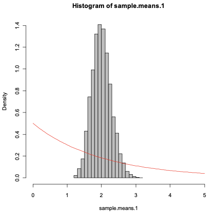

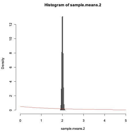
Sample 2 is much smaller than sample 1, thus it has a much denser distribution with more density in values closer to the mean of 2. Nevertheless, we can observe that the type of distribution is very similar and that is why the variance also changes at the same rate as the sample size.

> library(car)

> qq.plot(sample.means.1, envelope=.9999, col="black",

+ xlab="quantiles of standard normal distribution",

+ ylab="quantiles of sample means")

> library(car)

> qq.plot(sample.means.2, envelope=.9999, col="black",

+ xlab="quantiles of standard normal distribution",

+ ylab="quantiles of sample means")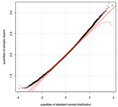

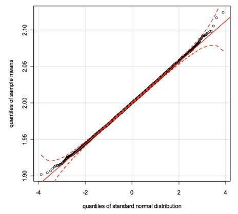
Both distributions are quite similar to the standard normal distribution as seen in the graph. Nevertheless, they are not the same and this is visible in the graph of sample 1 where the sample size is much larger and therefore the differences are more noticeable between exponential and normal distributions.

Computing Empirical Probabilities from Sample in File with R

# Take Sample and Compute Empirical Probabilities
> x=sample(seq(1:5),100,TRUE,c(0.1,0.2,0.4,0.2,0.1))
> table(x)/100
x
1 2 3 4 5
0.10 0.17 0.41 0.18 0.14

The maximum difference between sampled computed probability and original pmf here is 0.14–0.10 = 0.04.

The maximum is observed at x=3.

# Graph pmf sampling
> plot(seq(1:5),c(0.1,0.2,0.4,0.2,0.1),main=”PMF Sampling”,ylab=”p(x)”, xlab=”x”);lines(density(x))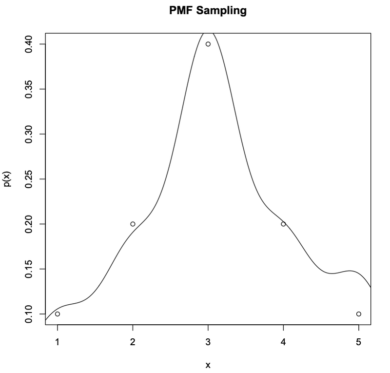

# Take Sample and Graph Histogram
> x=sample(seq(1:5),100,TRUE,c(0.1,0.2,0.4,0.2,0.1))
> hist(x, seq(0.5,5.5,1), freq=F, col=”gray”, main=”PMF Sampling”,ylab=”p(x)”, xlab=”x”);lines(density(x), col=”yellow”)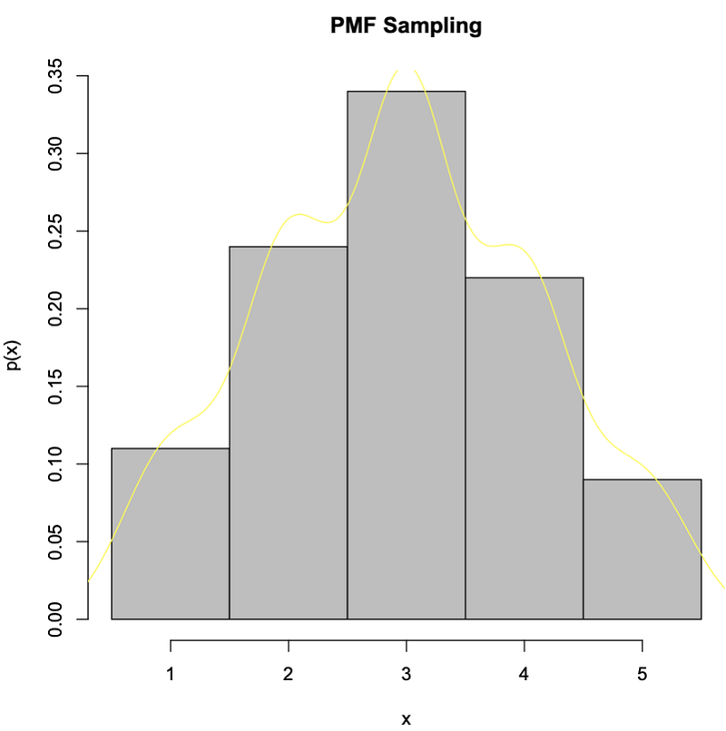

Computing for Distributions with R

# Boxplot cars=blue, trucks=red
> boxplot(bd[1:19,2],bd[20:38,2],names=c(“Car”,”Truck”), main=”Boxplot Stopping Distances for Vehicles”, ylab=”Stop Dist.”, col=c(“blue”,”red”))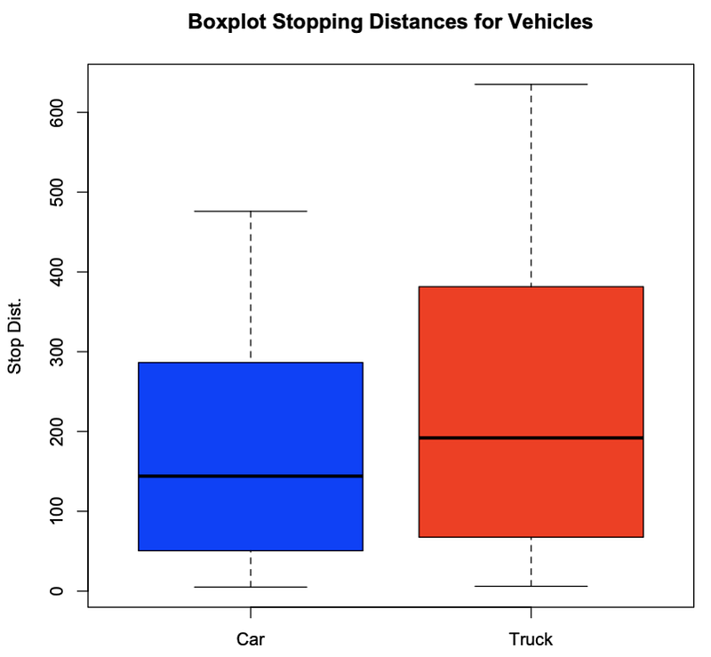

# Hypergeometric Probability of 2
> dhyper(2, 10, 20, 10)
# Hypergeometric Probability from 0 to 4
> sum(dhyper(0:4,10,20,10))
# Hypergeometric Probability from 2 to 8
> sum(dhyper(2:8,10,20,10))
# Hypergeometric Probability of 4 to 10(all)
> sum(dhyper(4:10,10,20,10))
[1] 0.1886719
[1] 0.8312529
[1] 0.9379412
[1] 0.4396606

The probability of 2 broken here is 0.1886719. The Probability of in between 2 or 8 broken here is 0.8312529. The Probability of less or equal to 4 broken here is 0.9379412. The Probability of 4 or more broken here is 0.4396606.

# Hypergeometric Probability of 2 broken out of 100 from 200 computers
> dhyper(2, 10, 200, 100)
# Binomial Approximation:
> dbinom(2,100,0.05)
[1] 0.05484615
[1] 0.08118177

The Hypergeometric Approximation here is 0.05484615. The Binomial Approximation to Hypergeometric here is 0.08118177.

Computing and Plotting for Proportions and Variances for Samples in Files with R

# Read Data
>cs=read.table(“http://sites.stat.psu.edu/~mga//401/Data/Concr.Strength.1s.Data.txt", header=T)
# Get Proportions
> attach(cs);sum(Str<=44)/length(Str);sum(Str>=47)/length(Str)
[1] 0.3125
[1] 0.21875

This population proportions of the category less or equal to 44 and more or equal to 47 represent the ratio of such categories when compared to the entire population. This shows the statistical variability of the population. From the data, we can determine that 31.25 percent of the data falls in the category of less or equal to 44 and that 21.875 percent of the data falls in the category of more or equal to 47, hence 46.875 percent of the data falls in between 44 and 47.

> x=c(rep(0,190),rep(1,160),rep(2,150))
> mean(x)
[1] 0.92
> sd(x)
[1] 0.8215533
> var(x)*(499/500)
[1] 0.6736

This sample has a mean of 0.92, a standard deviation of 0.8215533 and a population variance of 0.6736.

> y=sample(x, size=100)
> table(y)/100
y
0 1 2
0.32 0.39 0.29
> mean(y)
[1] 0.97
> var(y)
[1] 0.6152525
> sd(y)
[1] 0.7843803

The sample proportions here are 0=0.32, 1=0.39, 2=0.29. The mean of the sample is 0.97, the variance of the sample is 0.6152525 and the standard deviation of the sample is 0.7843803.

> attach(faithful); hist(waiting); stem(waiting)
The decimal point is 1 digit(s) to the right of the |
4 | 3
4 | 55566666777788899999
5 | 00000111111222223333333444444444
5 | 555555666677788889999999
6 | 00000022223334444
6 | 555667899
7 | 00001111123333333444444
7 | 555555556666666667777777777778888888888888889999999999
8 | 000000001111111111111222222222222333333333333334444444444
8 | 55555566666677888888999
9 | 00000012334
9 | 6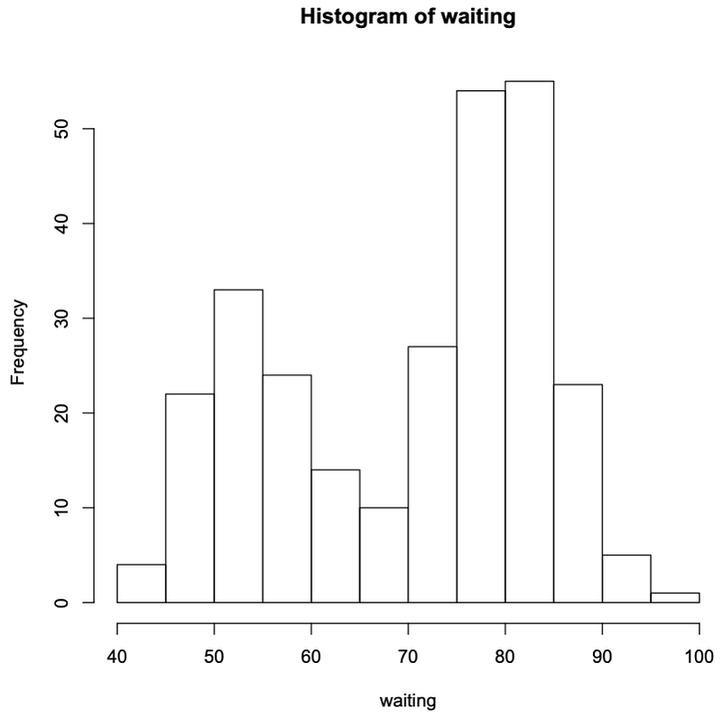

The stem and leaf display the data in a horizontal manner while the histogram does so vertically. Therefore the stem and leaf has the same shape as the histogram but rotated 90 degrees to the right.

> attach(faithful); hist(waiting, freq=F, col=”blue”, main=”Histogram of Old Faithful Data”); lines(density(waiting), col=”red”)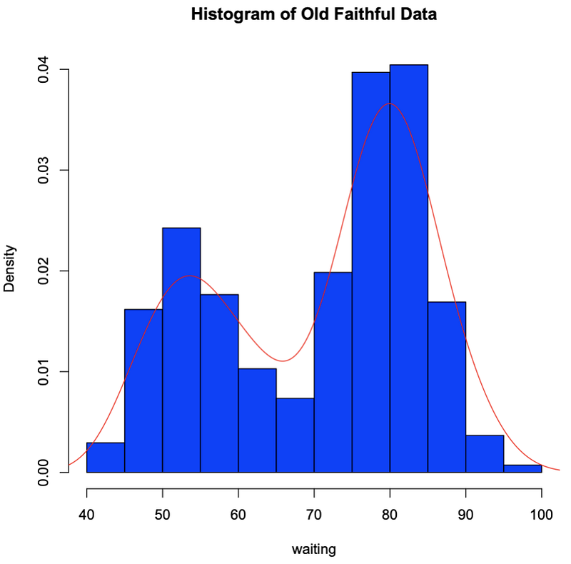

>cs=read.table(“http://sites.stat.psu.edu/~mga/401/Data/Temp.Long.Lat.txt", header=T)
> attach(cs); pairs(~City+JanTemp+Lat+Long,data=cs, main=”US Temperatures”)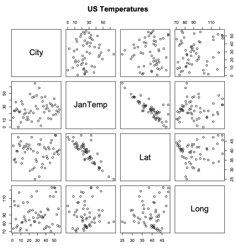

Latitude appears to be a better predictor of a city’s temperature for the plots comparing Temperatures with Latitude have a very clear correlation while the plots comparing Temperatures with Longitude do not have a very clear correlation.

>cs=read.table(“http://sites.stat.psu.edu/~mga/401/Data/Temp.Long.Lat.txt", header=T)
> library(scatterplot3d); attach(cs); scatterplot3d(JanTemp,Lat,Long, main=”US Temperatures”, angle=60, col.axis=”blue”,col.grid=”lightblue”,color=”red”,type=”h”,box=F)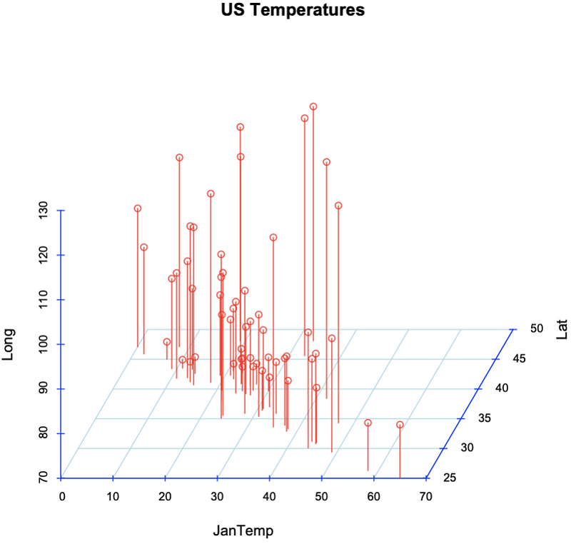

Latitude appears to be again the better predictor of a city’s temperature. This is visible in the graph in the fact that there seems to be a change in the correlation of Temperature data as the values from latitude are changed. With longitude, there is no obvious correlation between changes in longitude and changes in Temperature.

>bd=read.table(“http://sites.stat.psu.edu/~mga/401/Data/SpeedStopCarTruck.txt", header=T)
> attach(bd); plot(Speed,StopDist,pch=21, bg=c(“blue”,”red”)[unclass(Auto)], main=”Average Stopping Times”); legend(x=20, y=600, pch=c(21,21), col=c(“blue”,”red”), legend=c(“Car”, “Truck”))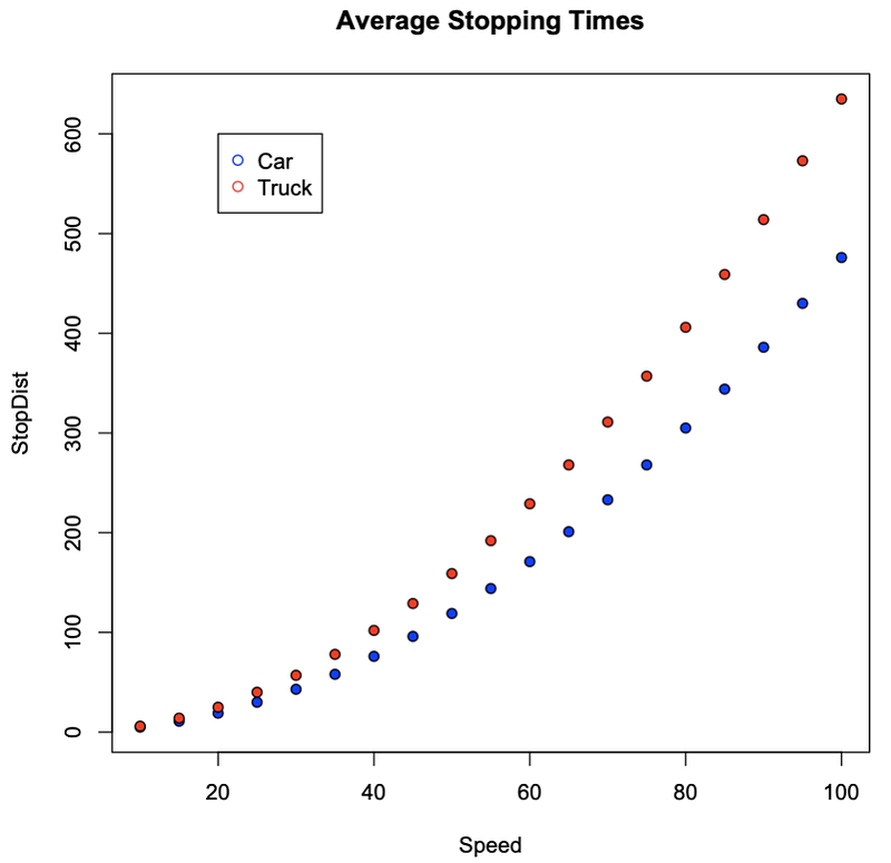

> # Read Data
>cs=read.table(“http://sites.stat.psu.edu/~mga/401/Data/RobotReactTime.txt", header=T)
> # Data for Robot 1
> Robot1=cs[1:22,]
> # Get Summary for Robot 1 Data
> summary(Robot1)
> # IQR
> quantile(Robot1[,1],.75)-quantile(Robot1[,1],.25)
> # 19th order value percentile
> ii=19
> ii=19;per=100*(ii-0.5)/length(Robot1[,1]);per
> # Approximate 90th percentile
Time Robot
Min. :27.05 Min. :1
1st Qu.:28.33 1st Qu.:1
Median :29.25 Median :1
Mean :29.22 Mean :1
3rd Qu.:30.07 3rd Qu.:1
Max. :31.44 Max. :1
75%
1.7425
[1] 84.09091
90%
30.57

The median of this distribution is 29.25, the 25th Percentile is 28.33, the 75th Percentile is 30.07, the Interquartile Range is 1.7425, the Percentile of 19th order is 84.09091, and the 90th Percentile is 30.57.

> # Data for Robot 2
> Robot2=cs[23:44,]
> # Get Summary
> summary(Robot2)
> # Get 90th percentile
> quantile(Robot2[,1],.9)
> # Get boxplot for Robot2 Data
> boxplot(Robot2)
Time Robot
Min. :27.67 Min. :2
1st Qu.:28.00 1st Qu.:2
Median :28.64 Median :2
Mean :28.81 Mean :2
3rd Qu.:29.52 3rd Qu.:2
Max. :30.93 Max. :2
90%
29.768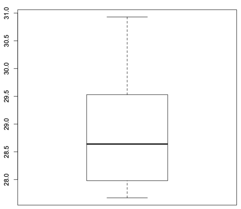

Time Robot
Min. :27.67 Min. :2
1st Qu.:28.00 1st Qu.:2
Median :28.64 Median :2
Mean :28.81 Mean :2
3rd Qu.:29.52 3rd Qu.:2
Max. :30.93 Max. :2
29.768
None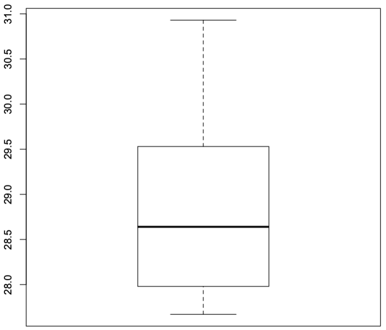

> # Create Engineer Vector
> engr=c(152,169,178,179,185,188,195,198,203,204,209,210,212,214)
> # Get the median
> median(engr)
> # Get the 25th percentile
> q1=quantile(engr,.25);q1
> # Get the 75th percentile
> q3=quantile(engr,.75);q3
> # Get the IQR
> q3-q1
> # Give 5000 raise
> engr=engr+5
> # Get new median
> median(engr)
> # Get new 25th percentile
> q1=quantile(engr,.25);q1
> # Get new 75th percentile
> q3=quantile(engr,.75);q3
> # Get new IQR
> q3-q1
> # Give 5% raise
> engr=engr*1.05
> # Get new median
> median(engr)
> # Get new 25th percentile
> q1=quantile(engr,.25);q1
> # Get new 75th percentile
> q3=quantile(engr,.75);q3
> # Get new IQR
> q3-q1
[1] 196.5
25%
180.5
75%
207.75
75%
27.25
[1] 201.5
25%
185.5
75%
212.75
75%
27.25
[1] 211.575
25%
194.775
75%
223.3875
75%
28.6125

The median of the first distribution is 196.5, the 25th percentile is 180.5, the 75th percentile is 207.75, the IQR is 27.25.

The median of the second distribution is 201.5, the 25th percentile is 185.5, the 75th percentile is 212.75, the IQR is 27.25.

The median of the third distribution is 211.575, the 25th percentile is 194.775, the 75th percentile is 223.3875, the IQR is 28.6125.

>mata=c(744,805,264,631,655,225,314,774,340,299,461,301,427,496,582,425,335,342,489,441,242,861,835,287,422)
>matb=c(1095,147,193,731,618,621,335,420,401,497,753,884,458,720,730,912,808,840,888,897,754,745,1086,210,1049,1012,279)
> mata=mata/100
> matb=matb/100
> boxplot(mata,matb)
> # Read Data
>cs=read.table(“http://sites.stat.psu.edu/~mga/401/Data/IgnitionTimesData.txt")
> # Store in Vectors
> a=cs[2:26,]
> b=cs[27:54,]
> # Boxplot
> boxplot(a[,2],b[,2])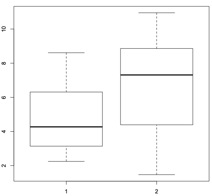

Material A, which is shown above the 1 in the comparative boxplot seems to have a shorter ignition time than Material B which is shown above the number 2 in the boxplot. It also seems like overall most of the values in Material A are closer to the minimum even though the IQR appears to be larger than for Material B. Therefore, Material A is more volatile and ignites faster than Material B.

Computing and Plotting for Finance and Economics with R

> prob=c(0.13,0.19,0.22,0.17,0.04,0.25)   #Event Probability

> rda=c(0.14,-0.07,0.23,0.06,0.03,0.05)       #RDA Return

> market=c(0.07,-0.07,0.09,0.06,-0.02,0.02) #Market Return

> e_rda=sum(prob*rda)     #E(RDA)=Σ(p*RDA)

> e_rda       #Expected Return RDA

[1] 0.0794

> e_market=sum(prob*market)    #E(Market)=Σ(p*Market)

> e_market       #Expected Return Market

[1] 0.03

> var_rda=sum(prob*(rda-e_rda)^2)   #σ2(RDA)=Σ(p*(RDA-E(RDA))^2)

> var_rda       #Variance RDA

[1] 0.01008564

> var_market=sum(prob*(market-e_market)^2) #σ2(Market)=Σ(p*(Market-#E(Market))^2)

> var_market      #Variance Market

[1] 0.003178

> std_rda=sqrt(var_rda)     #σ(RDA)=(σ2(RDA))^1/2

> std_rda       #Standard Deviation RDA

[1] 0.1004273

> std_market=sqrt(var_market)                  #σ(Market)=(σ2(Market))^1/2

> std_market      #Standard Deviation Market

[1] 0.05637375

> cov_rda_market=

+ sum(prob*((rda-e_rda)*(market-e_market))) #σ(RDA,Market)=Σ(p*((RDA-#E(RDA)*(Market-E(Market)))

> cov_rda_market      #Covariance RDA & Market

[1] 0.005215

> corr_rda_market=

+ cov_rda_market/(std_rda*std_market)  #corr(RDA,Market)= #σ(RDA,Market)/    #(σ(RDA)* σ(Market))

> corr_rda_market      #Correlation RDA & Market

[1] 0.92114

> b=(cov_rda_market/var_market)   #β=(σ(RDA,Market)/σ(Market))

> b  #Beta RDA with Market

[1] 1.640969

> rf=(-e_rda+b*e_market)/(b-1)   #Rf=(-E(Ri)+β*E(Rm))/(β-1)

> rf        #Risk Free Rate

[1] -0.04707079

The Risk-Free Rate of this option is -4.71%.

> C=c(6.95,5.9,4.45,3.8,4.2,3.2,2.13,2,1.2,0.85) #Call Price

> P=c(0.85,0.95,1.1,1.55,1.7,1.9,2.3,3.8,5.2,5.7) #Put Price

> K=c(32.5,34,35,36,37.5,39,40,41,42.5,44)  #Strike Price

> T=114/360        #Time (years)

> St=40.91        #Stock Price

> log(exp(1),base=exp(1))     #Verify Log as ln

[1] 1

> r=(log((-C+P+St)/K, base=exp(1)))/-T   #r=(ln((-C+P+St)/K)/-T

> r         #Annual interest rates

[1] -0.21683562 -0.17698953 -0.22292082 -0.22511537

-0.07571656

[6] -0.04901042 -0.08413241 -0.12903479 -0.17417814

-0.12385488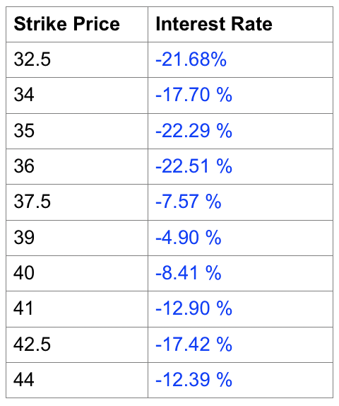

> Rf=0.02        #Risk Free Rate (%)

> T=6/12        #Time (years)

> K=93        #Strike Price

> C=6.479        #Call

> P=9.334        #Put

> X=(850:950)/10  #Stock Prices from 85                                                          #to 95,increments 0.1

> St=C-P+K*exp(-Rf*T)      #St=C-P+K*exp(-Rf*T)

> St         #Stock Worth

[1] 89.21963

> Profit=rep(0,101)      #Profits empty array

> for(i in 1:101)

+ if(X[i]<St){Profit[i]=(-X[i]+C-P)/exp(-Rf*T)+K

+ } else {Profit[i]=(X[i]-C+P)/exp(-Rf*T)-K}  #For each element if       #Price<Stock Worth       #then sell stock buy     #call sell put,   #discount and add    #Strike Price.         #Otherwise Profit         #Equals opposite.

> Profit        #Profit for each Price

[1] 4.26204257 4.16103755 4.06003254 3.95902752

3.85802250

[6] 3.75701749 3.65601247 3.55500745 3.45400244

3.35299742

[11] 3.25199240 3.15098739 3.04998237 2.94897735

2.84797234

[16] 2.74696732 2.64596230 2.54495729 2.44395227

2.34294725

[21] 2.24194224 2.14093722 2.03993220 1.93892719

1.83792217

[26] 1.73691715 1.63591214 1.53490712 1.43390210

1.33289709

[31] 1.23189207 1.13088705 1.02988204 0.92887702

0.82787200

[36] 0.72686699 0.62586197 0.52485695 0.42385194

0.32284692

[41] 0.22184190 0.12083689 0.01983187 0.08117315

0.18217816

[46] 0.28318318 0.38418820 0.48519321 0.58619823

0.68720325

[51] 0.78820826 0.88921328 0.99021830 1.09122331

1.19222833

[56] 1.29323335 1.39423836 1.49524338 1.59624840

1.69725341

[61] 1.79825843 1.89926345 2.00026847 2.10127348

2.20227850

[66] 2.30328352 2.40428853 2.50529355 2.60629857

2.70730358

[71] 2.80830860 2.90931362 3.01031863 3.11132365

3.21232867

[76] 3.31333368 3.41433870 3.51534372 3.61634873

3.71735375

[81] 3.81835877 3.91936378 4.02036880 4.12137382

4.22237883

[86] 4.32338385 4.42438887 4.52539388 4.62639890

4.72740392

[91] 4.82840893 4.92941395 5.03041897 5.13142398

5.23242900

[96] 5.33343402 5.43443903 5.53544405 5.63644907

5.73745408

[101] 5.83845910

> plot(X,Profit,type="o",col="blue",

+ xlab=”Stock Price($)",ylab="Profit per Stock ($)",

+ main="Arbitrage Profit vs. Stock Price")  #Plot Profit vs. Price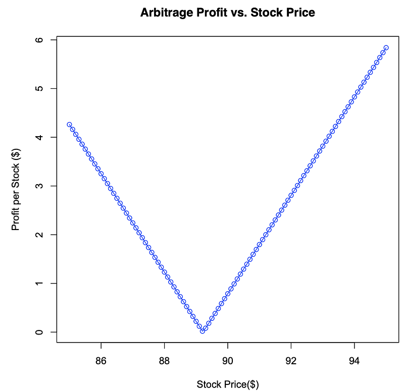

> T_a=4.75        #Maturity (Bond A)

> T_b=5        #Maturity (Bond B)

> i_a=1.6/100        #Interest (Bond A)

> i_b=1.7/100       #Interest (Bond B)

> t=0.5        #Time to Convergence

> i=(0:60)/1000       #Interest rates 0-6%

> Pta=exp(-T_a*i_a)      #P(A)=                                  #e^(-i(A)*T(A))

> Pta         #Price money (Bond A)

[1] 0.9268162

> Ptb=exp(-T_b*i_b)      #P(t)(B)=                                  #e^(-i(B)*T(B))

> Ptb         #Price money (Bond B)

[1] 0.9185123

> Capital=400000000      #Capital to Invest

> Short_1=Capital*Pta      #Go Short with Capital            #on 4.75yr bond

> Short_1        #Money from Short

[1] 370726483

> Long1=Short_1/Ptb      #Go Long with money                             #from Short on 5yr                                        #bond

> Long1        #Money on Long

[1] 403616249

> Pta2=exp(-i*(T_a-t))      #P(t)(A)=                                  #e^(-i(A)*T(A)-t)

> Pta2  #Price money varying i

[1] 1.0000000 0.9957590 0.9915360 0.9873309

0.9831437 0.9789742

[7] 0.9748224 0.9706882 0.9665715 0.9624723

0.9583905 0.9543259

[13] 0.9502787 0.9462486 0.9422355 0.9382395

0.9342605 0.9302983

[19] 0.9263529 0.9224243 0.9185123 0.9146169

0.9107380 0.9068756

[25] 0.9030296 0.8991998 0.8953863 0.8915890

0.8878078 0.8840426

[31] 0.8802934 0.8765601 0.8728426 0.8691409

0.8654549 0.8617845

[37] 0.8581297 0.8544904 0.8508665 0.8472580

0.8436648 0.8400868

[43] 0.8365241 0.8329764 0.8294437 0.8259261

0.8224233 0.8189355

[49] 0.8154624 0.8120040 0.8085603 0.8051312

0.8017167 0.7983166

[55] 0.7949310 0.7915597 0.7882027 0.7848599

0.7815314 0.7782169

[61] 0.7749165

> Ptb2=exp(-i*(T_b-t))      #P(t)(B)=                                  #e^(-i(B)*T(B)-t)

> Ptb2  #Price money varying i

[1] 1.0000000 0.9955101 0.9910404 0.9865907

0.9821610 0.9777512

[7] 0.9733612 0.9689910 0.9646403 0.9603092

0.9559975 0.9517052

[13] 0.9474321 0.9431782 0.9389435 0.9347277

0.9305309 0.9263529

[19] 0.9221937 0.9180531 0.9139312 0.9098277

0.9057427 0.9016760

[25] 0.8976276 0.8935973 0.8895852 0.8855911

0.8816148 0.8776565

[31] 0.8737159 0.8697930 0.8658877 0.8620000

0.8581297 0.8542768

[37] 0.8504412 0.8466228 0.8428216 0.8390374

0.8352702 0.8315199

[43] 0.8277865 0.8240698 0.8203699 0.8166865

0.8130196 0.8093693

[49] 0.8057353 0.8021176 0.7985162 0.7949310

0.7913618 0.7878087

[55] 0.7842715 0.7807502 0.7772447 0.7737550

0.7702809 0.7668224

[61] 0.7633795

> Short2=Capital*Pta2      #Go Short with Capital          #on Bond A with new                   #price of money

> Short2        #Money from Short

[1] 400000000 398303607 396614409 394932375

393257474 391589676

[7] 389928952 388275270 386628602 384988917

383356186 381730380

[13] 380111468 378499422 376894213 375295812

373704189 372119317

[19] 370541166 368969707 367404914 365846756

364295207 362750238

[25] 361211821 359679928 358154532 356635605

355123120 353617050

[31] 352117366 350624043 349137053 347656369

346181965 344713814

[37] 343251889 341796164 340346613 338903209

337465927 336034740

[43] 334609623 333190550 331777495 330370432

328969337 327574185

[49] 326184948 324801604 323424127 322052491

320686672 319326646

[55] 317972387 316623872 315281076 313943975

312612545 311286761

[61] 309966599

> Long2=Long1*Ptb2      #Go Long with Money                                       #from Long on 5yr bond                                             #with new Price of                           #money

> Long2        #Money on long

[1] 403616249 401804056 400000000 398204044

396416152 394636287

[7] 392864413 391100495 389344497 387596383

385856117 384123666

[13] 382398993 380682063 378972843 377271296

375577389 373891088

[19] 372212358 370541166 368877477 367221257

365572474 363931094

[25] 362297083 360670409 359051039 357438939

355834077 354236421

[31] 352645939 351062597 349486365 347917209

346355099 344800003

[37] 343251889 341710725 340176482 338649127

337128629 335614959

[43] 334108085 332607976 331114603 329627934

328147941 326674593

[49] 325207860 323747712 322294121 320847056

319406488 317972387

[55] 316544726 315123475 313708606 312300088

310897895 309501998

[61] 308112368

> Profit=rep(0,61)      #Empty Profits array

> for(j in 1:61)

+ if(Long2[j]>Short2[j]) {

+ Profit[j]=Long2[j]-Short2[j]

+ } else {Profit[j]=Short2[j]-Long2[j]}   #For each interest                                       #rate, make sure                                          #Profit>0 and                       #Profit=Long-Short  #otherwise                                                             #Profit=Short-Long

> Profit        #Profits for each i

[1] 3616248.71 3500448.69 3385590.85 3271669.17

3158677.66

[6] 3046610.36 2935461.36 2825224.77 2715894.75

2607465.49

[11] 2499931.18 2393286.10 2287524.52 2182640.76

2078629.16

[16] 1975484.12 1873200.04 1771771.38 1671192.61

1571458.24

[21] 1472562.82 1374500.91 1277267.14 1180856.12

1085262.54

[26]  990481.09  896506.50  803333.52  710956.96

619371.63

[31]  528572.38  438554.09  349311.68  260840.08

173134.26

[36]   86189.23       0.00   85438.36  170130.77

254082.11

[41]  337297.25  419781.01  501538.19  582573.56

662891.88

[46]  742497.85  821396.17  899591.50  977088.48

1053891.71

[51] 1130005.78 1205435.24 1280184.61 1354258.41

1427661.10

[56] 1500397.13 1572470.93 1643886.89 1714649.39

1784762.76

[61] 1854231.34

> plot(i,Profit,type="o",col="orange",

+ xlab="Interest Rate",ylab="Net Position ($)",

+ main="Interest Rate Convergence

+ vs. Value of Position")     #Plot i’s vs. Profit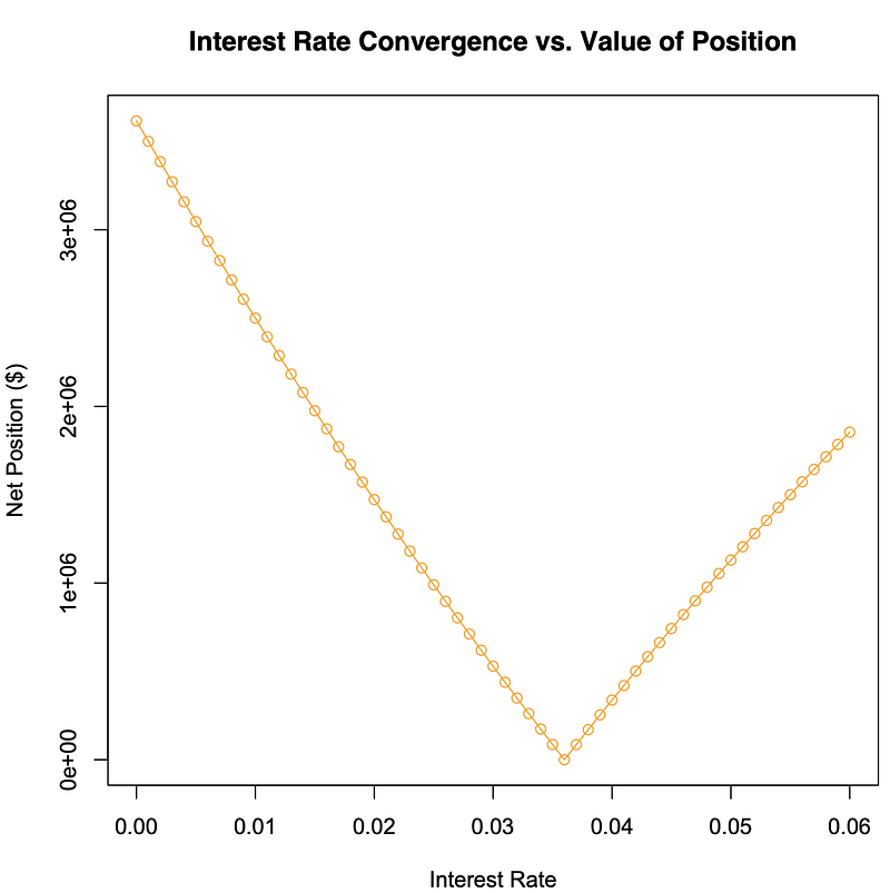

Computing for an Arbitrage Strategy with R

> face=500000000      #Face Value

> T1=10       #10 Yr. Bond Time

> T2=9.75       #9.75 Yr. Bond Time

> i2=0.02       #9.75 Yr. interest

> i=0.025       #Convergence “i”

> t=4/12       #Time to converge

> i1=(100:200)/10000     #10 Yr. interest

> i1        #10Yr. interest Rates

[1] 0.0100 0.0101 0.0102 0.0103 0.0104

0.0105 0.0106 0.0107

[9] 0.0108 0.0109 0.0110 0.0111 0.0112

0.0113 0.0114 0.0115

[17] 0.0116 0.0117 0.0118 0.0119 0.0120

0.0121 0.0122 0.0123

[25] 0.0124 0.0125 0.0126 0.0127 0.0128

0.0129 0.0130 0.0131

[33] 0.0132 0.0133 0.0134 0.0135 0.0136

0.0137 0.0138 0.0139

[41] 0.0140 0.0141 0.0142 0.0143 0.0144

0.0145 0.0146 0.0147

[49] 0.0148 0.0149 0.0150 0.0151 0.0152

0.0153 0.0154 0.0155

[57] 0.0156 0.0157 0.0158 0.0159 0.0160

0.0161 0.0162 0.0163

[65] 0.0164 0.0165 0.0166 0.0167 0.0168

0.0169 0.0170 0.0171
[73] 0.0172 0.0173 0.0174 0.0175 0.0176

0.0177 0.0178 0.0179

[81] 0.0180 0.0181 0.0182 0.0183 0.0184

0.0185 0.0186 0.0187

[89] 0.0188 0.0189 0.0190 0.0191 0.0192

0.0193 0.0194 0.0195

[97] 0.0196 0.0197 0.0198 0.0199 0.0200

> Pt2=exp(-i2*T2) #Pt(9.75yr)=

#e^- 0.02*9.75

> Pt2  #Price of Money for

[1] 0.8228347   #9.75 Yr. Bond

> Pt1b=exp(-i*(T1-t)) #Pt(10yrConv)=

#e^-0.025*10-1/3

> Pt1b  #Price of Money for

[1] 0.7853179 #10 Yr Bond Convrg.

> Pt2b=exp(-i*(T2-t))  #Pt(9.75yrConv)=

#e^-0.025*9.75-1/3

> Pt2b       #Price of Money for

[1] 0.7902415 #9.75 Yr Convrg.

> ShortPosition=face*Pt1b    #Value of Short=

#500m.*Pt(10yrConv)

> ShortPosition      #Value of Short

[1] 392658953

> Pt1=exp(-i1*T1)  #Pt(10yr)=

#e^-(0.01:0.02)*10

> Pt1        #Value of Money 10y

[1] 0.9048374 0.9039330 0.9030296 0.9021270

0.9012253

[6] 0.9003245 0.8994246 0.8985257 0.8976276

0.8967304

[11] 0.8958341 0.8949387 0.8940443 0.8931507

0.8922580

[16] 0.8913661 0.8904752 0.8895852 0.8886961

0.8878078

[21] 0.8869204 0.8860340 0.8851484 0.8842637

0.8833798

[26] 0.8824969 0.8816148 0.8807337 0.8798534

0.8789740

[31] 0.8780954 0.8772178 0.8763410 0.8754651

0.8745901

[36] 0.8737159 0.8728426 0.8719702 0.8710987

0.8702280

[41] 0.8693582 0.8684893 0.8676213 0.8667541

0.8658877

[46] 0.8650223 0.8641577 0.8632940 0.8624311

0.8615691

[51] 0.8607080 0.8598477 0.8589883 0.8581297

0.8572720

[56] 0.8564152 0.8555592 0.8547041 0.8538498

0.8529964

[61] 0.8521438 0.8512921 0.8504412 0.8495912

0.8487420

[66] 0.8478937 0.8470462 0.8461996 0.8453538

0.8445089

[71] 0.8436648 0.8428216 0.8419792 0.8411376

0.8402969

[76] 0.8394570 0.8386180 0.8377798 0.8369424

0.8361059

[81] 0.8352702 0.8344354 0.8336013 0.8327682

0.8319358

[86] 0.8311043 0.8302736 0.8294437 0.8286147

0.8277865

[91] 0.8269591 0.8261326 0.8253069 0.8244820

0.8236579

[96] 0.8228347 0.8220122 0.8211906 0.8203699

0.8195499

[101] 0.8187308

> Short=Pt1*face #Going Short 10yr

#bond=Pt(10yr)*500m

> Short       #Money from Short

[1] 452418709 451966516 451514776 451063487

450612649

[6] 450162261 449712324 449262836 448813798

448365209

[11] 447917068 447469374 447022129 446575330

446128978

[16] 445683072 445237612 444792597 444348026

443903900

[21] 443460218 443016980 442574184 442131831

441689920

[26] 441248451 440807423 440366836 439926690

439486983

[31] 439047715 438608887 438170498 437732546

437295032

[36] 436857956 436421316 435985113 435549346

435114014

[41] 434679118 434244656 433810628 433377034

432943874

[46] 432511147 432078852 431646989 431215557

430784557

[51] 430353988 429923849 429494140 429064861

428636011

[56] 428207589 427779595 427352029 426924891

426498179

[61] 426071894 425646036 425220602 424795594

424371011

[66] 423946852 423523117 423099806 422676917

422254452

[71] 421832408 421410787 420989587 420568807

420148449

[76] 419728510 419308992 418889892 418471212

418052950

[81] 417635106 417217679 416800670 416384078

415967902

[86] 415552142 415136797 414721868 414307354

413893253

[91] 413479567 413066294 412653434 412240987

411828952

[96] 411417329 411006117 410595317 410184927

409774947

[101] 409365377

> Long=Short/Pt2 #Long on 9.75 bond=

#Pt(9.75yr)*500m

> Long       #Money in Long

[1] 549829428 549279873 548730868 548182411

547634503

[6] 547087142 546540328 545994061 545448340

544903164

[11] 544358533 543814447 543270904 542727905

542185448

[16] 541643534 541102161 540561329 540021038

539481287

[21] 538942075 538403403 537865268 537327672

536790613

[26] 536254091 535718105 535182654 534647739

534113359

[31] 533579512 533046199 532513420 531981172

531449457

[36] 530918273 530387620 529857498 529327905

528798842

[41] 528270307 527742301 527214823 526687871

526161447

[46] 525635548 525110175 524585328 524061005

523537205

[51] 523013930 522491177 521968947 521447239

520926053

[56] 520405387 519885242 519365616 518846510

518327923

[61] 517809854 517292303 516775270 516258753

515742752

[66] 515227267 514712297 514197842 513683901

513170474

[71] 512657560 512145159 511633270 511121892

510611026

[76] 510100670 509590824 509081488 508572661

508064343

[81] 507556532 507049229 506542434 506036144

505530361

[86] 505025084 504520311 504016043 503512279

503009018

[91] 502506260 502004005 501502252 501001001

500500250

[96] 500000000 499500250 499000999 498502248

498003995

[101] 497506240

> LongPosition=Long/Pt2b #Value of Long =

#Money from Going

#long on 9.75 yr

#/Pt(9.75yrConv)

> LongPosition      #Value of Long

[1] 695773910 695078484 694383752 693689716

692996373

[6] 692303723 691611765 690920499 690229924

689540039

[11] 688850844 688162337 687474519 686787388

686100944

[16] 685415186 684730113 684045725 683362021

682679001

[21] 681996663 681315007 680634033 679953739

679274125

[26] 678595191 677916935 677239357 676562456

675886231

[31] 675210683 674535810 673861611 673188086

672515235

[36] 671843056 671171548 670500712 669830547

669161051

[41] 668492224 667824066 667156576 666489753

665823596

[46] 665158106 664493280 663829119 663165621

662502787

[51] 661840616 661179106 660518257 659858069

659198541

[56] 658539672 657881461 657223909 656567013

655910774

[61] 655255191 654600264 653945991 653292372

652639406

[66] 651987093 651335431 650684422 650034062

649384353

[71] 648735293 648086882 647439119 646792004

646145535

[76] 645499713 644854536 644210003 643566115

642922871

[81] 642280269 641638310 640996993 640356316

639716280

[86] 639076883 638438126 637800007 637162525

636525681

[91] 635889474 635253902 634618966 633984664

633350996

[96] 632717962 632085560 631453791 630822652

630192145

[101] 629562268

> Profit=LongPosition-ShortPosition  #Profit=

#Money from Long –

#Cost from Short

> Profit       #Payoff

[1] 303114956 302419530 301724799 301030762

300337419

[6] 299644770 298952812 298261546 297570971

296881086

[11] 296191890 295503384 294815565 294128434

293441990

[16] 292756232 292071160 291386772 290703068

290020048

[21] 289337710 288656054 287975080 287294786

286615172

[26] 285936237 285257981 284580403 283903502

283227278

[31] 282551730 281876856 281202658 280529133

279856281

[36] 279184102 278512595 277841759 277171593

276502098

[41] 275833271 275165113 274497623 273830800

273164643

[46] 272499152 271834327 271170165 270506668

269843834

[51] 269181662 268520153 267859304 267199116

266539588

[56] 265880719 265222508 264564955 263908060

263251821

[61] 262596238 261941311 261287037 260633418

259980453

[66] 259328139 258676478 258025468 257375109

256725400

[71] 256076340 255427929 254780166 254133051

253486582

[76] 252840759 252195582 251551050 250907162

250263918

[81] 249621316 248979357 248338039 247697363

247057326

[86] 246417930 245779172 245141053 244503572

243866728

[91] 243230521 242594949 241960013 241325711

240692043

[96] 240059009 239426607 238794837 238163699

237533192

[101] 236903315

> plot(i1,Profit,

main="Arbitrage Strategy",

xlab="10 Year Bond Rate",

ylab="Profit ($)", type="o",

col="lightseagreen")   #Plot Profit vs. i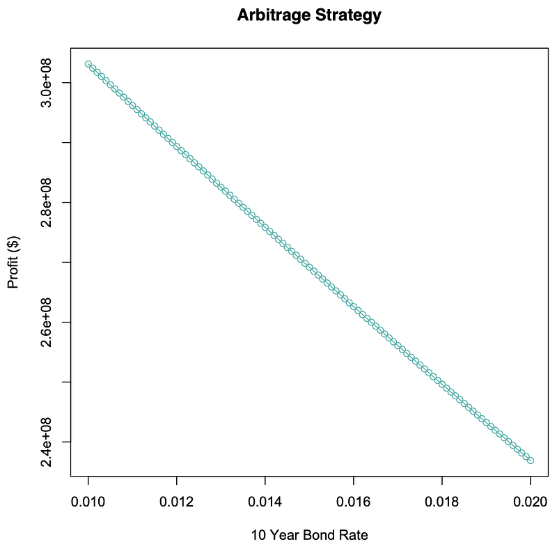

Forecasting Financials and Stock Prices with R

> p=c(0.1,0.2,0.2,0.1,0.2,0.2)    #Probabilities

> dmc=c(0.12,-0.06,-0.02,0.2,0.22,-0.1)  #Return DMC

> fdf=c(0.13,0.12,0.15,-0.2,0.3,0.18)  #Return FDF

> e_dmc=sum(p*dmc)     #E(DMC)=

# Σ(Probability*Return(DMC))

> e_dmc       #Expected Return DMC

[1] 0.04

> e_fdf=sum(p*fdf)     #E(FDF)=

# Σ(Probability*Return(FDF))

> e_fdf       #Expected Return FDF

[1] 0.143

> var_dmc=sum(p*(dmc-e_dmc)^2)   #σ(DMC)=

# Σ(Probability*(Return(DMC)          # -Expected(DMC))^2)

> var_dmc       #Variance DMC

[1] 0.01632

> var_fdf=sum(p*(fdf-e_fdf)^2)   #σ(FDF)=

# Σ(Probability*(Return(FDF)          # -Expected(FDF))^2)

> var_fdf       #Variance FDF

[1] 0.017101

> sd_dmc=sqrt(var_dmc)     #Standard Deviation(DMC)=

# (Variance(DMC))^(1/2)

> sd_dmc       #Standard Deviation DMC

[1] 0.1277498

> sd_fdf=sqrt(var_fdf)      #Standard Deviation(FDF)=         # (Variance(FDF))^(1/2)

> sd_fdf       #Standard Deviation FDF

[1] 0.1307708

> cov_dmc_fdf=sum(p*((dmc-e_dmc)*(fdf-e_fdf)))  #Covariance(DMC,FDF)=

# Σ(Probability*((Return(DMC)

# -Expected(DMC))*

# (Return(FDF)-

# Expected(FDF)))

> cov_dmc_fdf      #Covariance of DMC and FDF

[1] -6e-04

> corr_dmc_fdf = cov_dmc_fdf/(sd_dmc*sd_fdf) #Correlation(DMC,FDF)=

# Covariance(DMC,FDF)/

# (Standard Deviation(DMC)*

# Standard Deviation(FDF))

> corr_dmc_fdf      #Correlation DMC and FDF

[1] -0.03591538

The expected return for DMC here is 0.04, the variance for DMC is 0.01632, the standard deviation for DMC is 0.1277498.

The expected return for FDF is 0.143, the variance for FDF is 0.017101, the standard deviation for FDF is 0.1307708.

The covariance between DMC and FDF is -6*10^-4, and the correlation between DMC and FDF is -0.03591538.

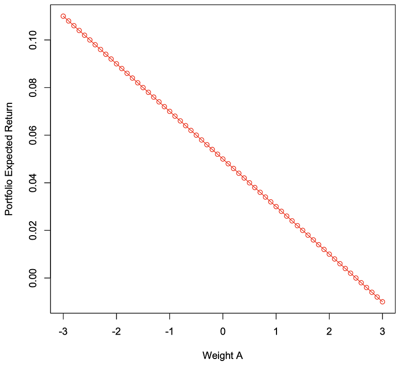
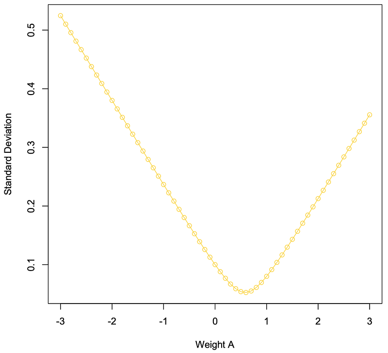
> weight_a=c(-30:30)/10     #Weight Commodity A

# from -3 to 3

> weight_a       #Weight Commodity A

[1] -3.0 -2.9 -2.8 -2.7 -2.6 -2.5 -2.4 -2.3

-2.2 -2.1 -2.0 -1.9

[13] -1.8 -1.7 -1.6 -1.5 -1.4 -1.3 -1.2 -1.1

-1.0 -0.9 -0.8 -0.7

[25] -0.6 -0.5 -0.4 -0.3 -0.2 -0.1  0.0  0.1

0.2  0.3  0.4  0.5

[37]  0.6  0.7  0.8  0.9  1.0  1.1  1.2  1.3

1.4  1.5  1.6  1.7

[49]  1.8  1.9  2.0  2.1  2.2  2.3  2.4  2.5

2.6  2.7  2.8  2.9

[61]  3.0

> weight_b=c(40:-20)/10     #Weight Commodity B

# from 4 to -2

> weight_b       #Weight Commodity B

[[1]  4.0  3.9  3.8  3.7  3.6  3.5  3.4  3.3

3.2  3.1  3.0  2.9

[13]  2.8  2.7  2.6  2.5  2.4  2.3  2.2  2.1

2.0  1.9  1.8  1.7

[25]  1.6  1.5  1.4  1.3  1.2  1.1  1.0  0.9

0.8  0.7  0.6  0.5

[37]  0.4  0.3  0.2  0.1  0.0 -0.1 -0.2 -0.3

-0.4 -0.5 -0.6 -0.7

[49] -0.8 -0.9 -1.0 -1.1 -1.2 -1.3 -1.4 -1.5

-1.6 -1.7 -1.8 -1.9

[61] -2.0

> comm_sda=0.08      #Standard Deviation           # Commodity A=8%

> comm_ea=0.03      #Expected Return

# Commodity A=3%

> comm_eb=0.05      #Expected Return

# Commodity B=5%

> comm_sdb=0.1      #Standard Deviation           # Commodity B=1%

> corr_ab=-0.3      #Correlation A&B=-0.3

> e_wab=(weight_a*comm_ea)+(weight_b*comm_eb) #Expected Return            # Portfolio=

# ((Weight A * Expected A)+

# (Weight B * Expected B))

> e_wab       #Expected Return A&B

[1]  1.100000e-01  1.080000e-01  1.060000e-01

1.040000e-01

[5]  1.020000e-01  1.000000e-01  9.800000e-02

9.600000e-02

[9]  9.400000e-02  9.200000e-02  9.000000e-02

8.800000e-02

[13]  8.600000e-02  8.400000e-02  8.200000e-02

8.000000e-02

[17]  7.800000e-02  7.600000e-02  7.400000e-02

7.200000e-02

[21]  7.000000e-02  6.800000e-02  6.600000e-02

6.400000e-02

[25]  6.200000e-02  6.000000e-02  5.800000e-02

5.600000e-02

[29]  5.400000e-02  5.200000e-02  5.000000e-02

4.800000e-02

[33]  4.600000e-02  4.400000e-02  4.200000e-02

4.000000e-02

[37]  3.800000e-02  3.600000e-02  3.400000e-02

3.200000e-02

[41]  3.000000e-02  2.800000e-02  2.600000e-02

2.400000e-02

[45]  2.200000e-02  2.000000e-02  1.800000e-02

1.600000e-02

[49]  1.400000e-02  1.200000e-02  1.000000e-02

8.000000e-03

[53]  6.000000e-03  4.000000e-03  2.000000e-03

-1.387779e-17

[57] -2.000000e-03 -4.000000e-03 -6.000000e-03

-8.000000e-03

[61] -1.000000e-02

> cov_ab=corr_ab*comm_sda*comm_sdb   #Covariance A&B=

# Correlation(A,B)*

# Standard Deviation(A)*

# Standard Deviation(B)

> cov_ab       #Covariance A&B

[1] -0.0024

> var_a=(comm_sda)^2     #σ(A)=(Standard            # Deviation A)^(1/2)

> var_a       #Variance Commodity A

[1] 0.0064

> var_b=(comm_sdb)^2     #σ(B)=(Standard

# Deviation B)^(1/2)

> var_b       #Variance Commodity B

[1] 0.01

> port_var=(weight_a^2*var_a+weight_b^2*var_b

+2*weight_a*weight_b*cov_ab)    #Portfolio Variance=

# ((WeightA^2*VarianceA) +

# (WeightB^2*VarianceB) +

# (2*WeightA*WeightB

# *Covariance(A,B))

> port_var       #Portfolio Variance

[1] 0.275200 0.260212 0.245648 0.231508

0.217792 0.204500

[7] 0.191632 0.179188 0.167168 0.155572

0.144400 0.133652

[13] 0.123328 0.113428 0.103952 0.094900

0.086272 0.078068

[19] 0.070288 0.062932 0.056000 0.049492

0.043408 0.037748

[25] 0.032512 0.027700 0.023312 0.019348

0.015808 0.012692

[31] 0.010000 0.007732 0.005888 0.004468

0.003472 0.002900

[37] 0.002752 0.003028 0.003728 0.004852

0.006400 0.008372

[43] 0.010768 0.013588 0.016832 0.020500

0.024592 0.029108

[49] 0.034048 0.039412 0.045200 0.051412

0.058048 0.065108

[55] 0.072592 0.080500 0.088832 0.097588

0.106768 0.116372

[61] 0.126400

> sd_ab=sqrt(port_var)     #Portfolio Standard           # Deviation=

# (Portfolio Variance)^(1/2)

> sd_ab       #Portfolio Standard Deviation

[1] 0.52459508 0.51010979 0.49562889 0.48115278

0.46668190

[6] 0.45221676 0.43775792 0.42330604 0.40886183

0.39442617

[11] 0.38000000 0.36558446 0.35118087 0.33679074

0.32241588

[16] 0.30805844 0.29372096 0.27940651 0.26511884

0.25086251

[21] 0.23664319 0.22246798 0.20834587 0.19428845

0.18031084

[26] 0.16643317 0.15268268 0.13909709 0.12572987

0.11265878

[31] 0.10000000 0.08793179 0.07673330 0.06684310

0.05892368

[36] 0.05385165 0.05245951 0.05502727 0.06105735

0.06965630

[41] 0.08000000 0.09149863 0.10376897 0.11656758

0.12973820

[46] 0.14317821 0.15681837 0.17061067 0.18452100

0.19852456

[51] 0.21260292 0.22674214 0.24093153 0.25516269

0.26942903

[56] 0.28372522 0.29804698 0.31239078 0.32675373

0.34113340

[61] 0.35552778

> plot(weight_a,e_wab,main="",

type="o", xlab="Weight A",

ylab="Portfolio Expected Return",col="red") #Plot Weight Commodity A

# from -3 to 3 vs.           # Expected REturn Portfolio

> plot(weight_a,sd_ab,main="",

type="o",xlab="Weight A", ylab="Standard

Deviation",col="gold",xlim=c(-3,3))    #Plot Weight Commodity A

# from -3 to 3 vs.

# Standard Deviation           # Portfolio

> dorsai_e=0.03      #Expected Return Dorsai=3%

> dorsai_sd=0.08       #Standard Deviation Dorsai=8%

> dfmc_e=0.05      #Expected Return DFMC=5%

> dfmc_sd=0.12      #Standard Deviation DFMC=12%

> weight_dorsai=17     #Weight Dorsai = 17

> weight_dfmc=-16      #Weight DFMC = -16

> var_dorsai=(dorsai_sd)^2    #σ(Dorsai)=(Standard           # Deviation Dorsai)^(1/2)

> var_dorsai      #Variance Dorsai

[1] 0.0064

> var_dfmc=(dfmc_sd)^2      #σ(DFMC)=(Standard           # Deviation DFMC)^(1/2)

> var_dfmc       #Variance DFMC

[1] 0.0144

> corr_dorsai_dfmc=(-90:90)/100   #Correlation Dorsai & DFMC          # from -.9 to .9

> corr_dorsai_dfmc     #Correlation Dorsai & DFMC

[1] -0.90 -0.89 -0.88 -0.87 -0.86 -0.85 -0.84

-0.83 -0.82

[10] -0.81 -0.80 -0.79 -0.78 -0.77 -0.76

-0.75 -0.74 -0.73

[19] -0.72 -0.71 -0.70 -0.69 -0.68 -0.67

-0.66 -0.65 -0.64

[28] -0.63 -0.62 -0.61 -0.60 -0.59 -0.58

-0.57 -0.56 -0.55

[37] -0.54 -0.53 -0.52 -0.51 -0.50 -0.49

-0.48 -0.47 -0.46

[46] -0.45 -0.44 -0.43 -0.42 -0.41 -0.40

-0.39 -0.38 -0.37

[55] -0.36 -0.35 -0.34 -0.33 -0.32 -0.31

-0.30 -0.29 -0.28

[64] -0.27 -0.26 -0.25 -0.24 -0.23 -0.22

-0.21 -0.20 -0.19

[73] -0.18 -0.17 -0.16 -0.15 -0.14 -0.13

-0.12 -0.11 -0.10

[82] -0.09 -0.08 -0.07 -0.06 -0.05 -0.04

-0.03 -0.02 -0.01

[91]  0.00  0.01  0.02  0.03  0.04  0.05

0.06  0.07  0.08

[100]  0.09  0.10  0.11  0.12  0.13  0.14

0.15  0.16  0.17

[109]  0.18  0.19  0.20  0.21  0.22  0.23

0.24  0.25  0.26

[118]  0.27  0.28  0.29  0.30  0.31  0.32

0.33  0.34  0.35

[127]  0.36  0.37  0.38  0.39  0.40  0.41

0.42  0.43  0.44

[136]  0.45  0.46  0.47  0.48  0.49  0.50

0.51  0.52  0.53

[145]  0.54  0.55  0.56  0.57  0.58  0.59

0.60  0.61  0.62

[154]  0.63  0.64  0.65  0.66  0.67  0.68

0.69  0.70  0.71

[163]  0.72  0.73  0.74  0.75  0.76  0.77

0.78  0.79  0.80

[172]  0.81  0.82  0.83  0.84  0.85  0.86

0.87  0.88  0.89

[181]  0.90

> cov_dorsai_dfmc=(corr_dorsai_dfmc)

*(dorsai_sd*dfmc_sd)     #Covariance Dorsai & DFMC =

# Correlation(Dorsai,DFMC)*

# Standard Deviation(Dorsai)*

# Standard Deviation(DFMC)

> cov_dorsai_dfmc      #Covariance Dorsai & DFMC

[1] -0.008640 -0.008544 -0.008448 -0.008352

-0.008256

[6] -0.008160 -0.008064 -0.007968 -0.007872

-0.007776

[11] -0.007680 -0.007584 -0.007488 -0.007392

-0.007296

[16] -0.007200 -0.007104 -0.007008 -0.006912

-0.006816

[21] -0.006720 -0.006624 -0.006528 -0.006432

-0.006336

[26] -0.006240 -0.006144 -0.006048 -0.005952

-0.005856

[31] -0.005760 -0.005664 -0.005568 -0.005472

-0.005376

[36] -0.005280 -0.005184 -0.005088 -0.004992

-0.004896

[41] -0.004800 -0.004704 -0.004608 -0.004512

-0.004416

[46] -0.004320 -0.004224 -0.004128 -0.004032

-0.003936

[51] -0.003840 -0.003744 -0.003648 -0.003552

-0.003456

[56] -0.003360 -0.003264 -0.003168 -0.003072

-0.002976

[61] -0.002880 -0.002784 -0.002688 -0.002592

-0.002496

[66] -0.002400 -0.002304 -0.002208 -0.002112

-0.002016

[71] -0.001920 -0.001824 -0.001728 -0.001632

-0.001536

[76] -0.001440 -0.001344 -0.001248 -0.001152

-0.001056

[81] -0.000960 -0.000864 -0.000768 -0.000672

-0.000576

[86] -0.000480 -0.000384 -0.000288 -0.000192

-0.000096

[91]  0.000000  0.000096  0.000192  0.000288

0.000384

[96]  0.000480  0.000576  0.000672  0.000768

0.000864

[101]  0.000960  0.001056  0.001152  0.001248

0.001344

[106]  0.001440  0.001536  0.001632  0.001728

0.001824

[111]  0.001920  0.002016  0.002112  0.002208

0.002304

[116]  0.002400  0.002496  0.002592  0.002688

0.002784

[121]  0.002880  0.002976  0.003072  0.003168

0.003264

[126]  0.003360  0.003456  0.003552  0.003648

0.003744

[131]  0.003840  0.003936  0.004032  0.004128

0.004224

[136]  0.004320  0.004416  0.004512  0.004608

0.004704

[141]  0.004800  0.004896  0.004992  0.005088

0.005184

[146]  0.005280  0.005376  0.005472  0.005568

0.005664

[151]  0.005760  0.005856  0.005952  0.006048

0.006144

[156]  0.006240  0.006336  0.006432  0.006528

0.006624

[161]  0.006720  0.006816  0.006912  0.007008

0.007104

[166]  0.007200  0.007296  0.007392  0.007488

0.007584

[171]  0.007680  0.007776  0.007872  0.007968

0.008064

[176]  0.008160  0.008256  0.008352  0.008448

0.008544

[181]  0.008640

>var_port=(weight_dorsai^2)*(var_dorsai)

+(weight_dfmc^2)*(var_dfmc)

+2*(weight_dorsai*weight_dfmc*cov_dorsai_dfmc) #Variance Portfolio=

# (Weight(Dorsai)^2*

# Variance(Dorsai)) +

# (Weight(DFMC)^2*

# Variance(DFMC)) +

# 2*(Weight(Dorsai)*

# Weight(DFMC)*

# Covariance(Dorsai,DFMC)

> var_port       #Variance Portfolio

[1] 10.236160 10.183936 10.131712 10.079488

10.027264

[6]  9.975040  9.922816  9.870592  9.818368

9.766144

[11]  9.713920  9.661696  9.609472  9.557248

9.505024

[16]  9.452800  9.400576  9.348352  9.296128

9.243904

[21]  9.191680  9.139456  9.087232  9.035008

8.982784

[26]  8.930560  8.878336  8.826112  8.773888

8.721664

[31]  8.669440  8.617216  8.564992  8.512768

8.460544

[36]  8.408320  8.356096  8.303872  8.251648

8.199424

[41]  8.147200  8.094976  8.042752  7.990528

7.938304

[46]  7.886080  7.833856  7.781632  7.729408

7.677184

[51]  7.624960  7.572736  7.520512  7.468288

7.416064

[56]  7.363840  7.311616  7.259392  7.207168

7.154944

[61]  7.102720  7.050496  6.998272  6.946048

6.893824

[66]  6.841600  6.789376  6.737152  6.684928

6.632704

[71]  6.580480  6.528256  6.476032  6.423808

6.371584

[76]  6.319360  6.267136  6.214912  6.162688

6.110464

[81]  6.058240  6.006016  5.953792  5.901568

5.849344

[86]  5.797120  5.744896  5.692672  5.640448

5.588224

[91]  5.536000  5.483776  5.431552  5.379328

5.327104

[96]  5.274880  5.222656  5.170432  5.118208

5.065984

[101]  5.013760  4.961536  4.909312  4.857088

4.804864

[106]  4.752640  4.700416  4.648192  4.595968

4.543744

[111]  4.491520  4.439296  4.387072  4.334848

4.282624

[116]  4.230400  4.178176  4.125952  4.073728

4.021504

[121]  3.969280  3.917056  3.864832  3.812608

3.760384

[126]  3.708160  3.655936  3.603712  3.551488

3.499264

[131]  3.447040  3.394816  3.342592  3.290368

3.238144

[136]  3.185920  3.133696  3.081472  3.029248

2.977024

[141]  2.924800  2.872576  2.820352  2.768128

2.715904

[146]  2.663680  2.611456  2.559232  2.507008

2.454784

[151]  2.402560  2.350336  2.298112  2.245888

2.193664

[156]  2.141440  2.089216  2.036992  1.984768

1.932544

[161]  1.880320  1.828096  1.775872  1.723648

1.671424

[166]  1.619200  1.566976  1.514752  1.462528

1.410304

[171]  1.358080  1.305856  1.253632  1.201408

1.149184

[176]  1.096960  1.044736  0.992512  0.940288

0.888064

[181]  0.835840

> sd_port=sqrt(var_port)    #Standard DeviationPortfolio

# =(Variance Portfolio)^(1/2)

> sd_port       #Standard Deviation Portfolio

[1] 3.1993999 3.1912280 3.1830350 3.1748209

3.1665855

[6] 3.1583287 3.1500502 3.1417498 3.1334275

3.1250830

[11] 3.1167162 3.1083269 3.0999148 3.0914799

3.0830219

[16] 3.0745406 3.0660359 3.0575075 3.0489552

3.0403789

[21] 3.0317784 3.0231533 3.0145036 3.0058290

2.9971293

[26] 2.9884043 2.9796537 2.9708773 2.9620749

2.9532463

[31] 2.9443913 2.9355095 2.9266008 2.9176648

2.9087014

[36] 2.8997103 2.8906913 2.8816440 2.8725682

2.8634636

[41] 2.8543300 2.8451671 2.8359746 2.8267522

2.8174996

[46] 2.8082165 2.7989026 2.7895577 2.7801813

2.7707732

[51] 2.7613330 2.7518605 2.7423552 2.7328169

2.7232451

[56] 2.7136396 2.7040000 2.6943259 2.6846169

2.6748727

[61] 2.6650929 2.6552770 2.6454247 2.6355356

2.6256093

[66] 2.6156452 2.6056431 2.5956024 2.5855228

2.5754037

[71] 2.5652446 2.5550452 2.5448049 2.5345232

2.5241997

[76] 2.5138337 2.5034249 2.4929725 2.4824762

2.4719353

[81] 2.4613492 2.4507174 2.4400393 2.4293143

2.4185417

[86] 2.4077209 2.3968513 2.3859321 2.3749627

2.3639425

[91] 2.3528706 2.3417464 2.3305690 2.3193378

2.3080520

[96] 2.2967107 2.2853131 2.2738584 2.2623457

2.2507741

[101] 2.2391427 2.2274506 2.2156967 2.2038802

2.1920000

[106] 2.1800550 2.1680443 2.1559666 2.1438209

2.1316060

[111] 2.1193206 2.1069637 2.0945338 2.0820298

2.0694502

[116] 2.0567936 2.0440587 2.0312440 2.0183478

2.0053688

[121] 1.9923052 1.9791554 1.9659176 1.9525901

1.9391710

[126] 1.9256583 1.9120502 1.8983445 1.8845392

1.8706320

[131] 1.8566206 1.8425026 1.8282757 1.8139372

1.7994844

[136] 1.7849146 1.7702248 1.7554122 1.7404735

1.7254055

[141] 1.7102047 1.6948675 1.6793904 1.6637692

1.6480000

[146] 1.6320784 1.6160000 1.5997600 1.5833534

1.5667750

[151] 1.5500194 1.5330806 1.5159525 1.4986287

1.4811023

[156] 1.4633660 1.4454121 1.4272323 1.4088179

1.3901597

[161] 1.3712476 1.3520710 1.3326185 1.3128778

1.2928356

[166] 1.2724779 1.2517891 1.2307526 1.2093502

1.1875622

[171] 1.1653669 1.1427406 1.1196571 1.0960876

1.0720000

[176] 1.0473586 1.0221233 0.9962490 0.9696845

0.9423715

[181] 0.9142429

> plot(corr_dorsai_dfmc,sd_port,

main="", xlab="Correlation",

ylab="Portfolio Standard Deviation",

type="o", col="purple",ylim=c(0,3.5))  #Plot Correlation vs.           # Standard Deviation           # Portfolio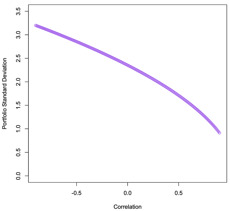

> klm_mean=0.05      #Mean(KLM expected Return)

> investment=100000     #Initial Investment

> min=95000       #Min=(At least 95000)

> max=107000      #Max=(At most 107000)

> sd_returns=(1:25)/100     #Standard Deviation

# from 1 to 25 percent

> sd_returns      #Standard Deviation(Returns)

[1] 0.010 0.011 0.012 0.013 0.014 0.015 0.016

0.017 0.018

[10] 0.019 0.020 0.021 0.022 0.023 0.024 0.025

0.026 0.027

[19] 0.028 0.029 0.030 0.031 0.032 0.033 0.034

0.035 0.036

[28] 0.037 0.038 0.039 0.040 0.041 0.042 0.043

0.044 0.045

[37] 0.046 0.047 0.048 0.049 0.050 0.051 0.052

0.053 0.054

[46] 0.055 0.056 0.057 0.058 0.059 0.060 0.061

0.062 0.063

[55] 0.064 0.065 0.066 0.067 0.068 0.069 0.070

0.071 0.072

[64] 0.073 0.074 0.075 0.076 0.077 0.078 0.079

0.080 0.081

[73] 0.082 0.083 0.084 0.085 0.086 0.087 0.088

0.089 0.090

[82] 0.091 0.092 0.093 0.094 0.095 0.096 0.097

0.098 0.099

[91] 0.100 0.101 0.102 0.103 0.104 0.105 0.106

0.107 0.108

[100] 0.109 0.110 0.111 0.112 0.113 0.114 0.115

0.116 0.117

[109] 0.118 0.119 0.120 0.121 0.122 0.123 0.124

0.125 0.126

[118] 0.127 0.128 0.129 0.130 0.131 0.132 0.133

0.134 0.135

[127] 0.136 0.137 0.138 0.139 0.140 0.141 0.142

0.143 0.144

[136] 0.145 0.146 0.147 0.148 0.149 0.150 0.151

0.152 0.153

[145] 0.154 0.155 0.156 0.157 0.158 0.159 0.160

0.161 0.162

[154] 0.163 0.164 0.165 0.166 0.167 0.168 0.169

0.170 0.171

[163] 0.172 0.173 0.174 0.175 0.176 0.177 0.178

0.179 0.180

[172] 0.181 0.182 0.183 0.184 0.185 0.186 0.187

0.188 0.189

[181] 0.190 0.191 0.192 0.193 0.194 0.195 0.196

0.197 0.198

[190] 0.199 0.200 0.201 0.202 0.203 0.204 0.205

0.206 0.207

[199] 0.208 0.209 0.210 0.211 0.212 0.213 0.214

0.215 0.216

[208] 0.217 0.218 0.219 0.220 0.221 0.222 0.223

0.224 0.225

[217] 0.226 0.227 0.228 0.229 0.230 0.231 0.232

0.233 0.234

[226] 0.235 0.236 0.237 0.238 0.239 0.240 0.241

0.242 0.243

[235] 0.244 0.245 0.246 0.247 0.248 0.249 0.250

> above_min=1-pnorm(-0.05,klm_mean,

sd_returns,lower.tail=TRUE,log.p=FALSE)  #Probability At least 95000=

# 1-Probability that a given          # Normal Distributed Function         # will have values lower than         # than that of less 5 percent         # its original value

> above_min       #Probabilities at least 95000         # as Standard Deviation goes          # from 1 to 25 percent

[1] 1.0000000 1.0000000 1.0000000 1.0000000

1.0000000

[6] 1.0000000 1.0000000 1.0000000 1.0000000

0.9999999

[11] 0.9999997 0.9999990 0.9999973 0.9999931

0.9999845

[16] 0.9999683 0.9999400 0.9998938 0.9998225

0.9997179

[21] 0.9995709 0.9993719 0.9991110 0.9987785

0.9983652

[26] 0.9978626 0.9972634 0.9965611 0.9957505

0.9948279

[31] 0.9937903 0.9926365 0.9913660 0.9899796

0.9884787

[36] 0.9868659 0.9851442 0.9833173 0.9813896

0.9793655

[41] 0.9772499 0.9750479 0.9727648 0.9704059

0.9679765

[46] 0.9654818 0.9629272 0.9603178 0.9576585

0.9549543

[51] 0.9522096 0.9494292 0.9466172 0.9437778

0.9409149

[56] 0.9380321 0.9351330 0.9322208 0.9292987

0.9263697

[61] 0.9234363 0.9205012 0.9175667 0.9146352

0.9117085

[66] 0.9087888 0.9058776 0.9029768 0.9000877

0.8972117

[71] 0.8943502 0.8915043 0.8886751 0.8858635

0.8830704

[76] 0.8802966 0.8775428 0.8748097 0.8720978

0.8694077

[81] 0.8667397 0.8640944 0.8614720 0.8588728

0.8562971

[86] 0.8537451 0.8512169 0.8487127 0.8462325

0.8437766

[91] 0.8413447 0.8389371 0.8365537 0.8341944

0.8318593

[96] 0.8295481 0.8272609 0.8249975 0.8227578

0.8205416

[101] 0.8183489 0.8161795 0.8140332 0.8119098

0.8098091

[106] 0.8077310 0.8056752 0.8036416 0.8016300

0.7996400

[111] 0.7976716 0.7957245 0.7937985 0.7918933

0.7900088

[116] 0.7881446 0.7863006 0.7844766 0.7826723

0.7808874

[121] 0.7791218 0.7773753 0.7756475 0.7739383

0.7722474

[126] 0.7705747 0.7689198 0.7672826 0.7656628

0.7640603

[131] 0.7624747 0.7609060 0.7593538 0.7578179

0.7562982

[136] 0.7547945 0.7533064 0.7518339 0.7503767

0.7489346

[141] 0.7475075 0.7460950 0.7446971 0.7433135

0.7419441

[146] 0.7405887 0.7392470 0.7379189 0.7366042

0.7353028

[151] 0.7340145 0.7327390 0.7314763 0.7302261

0.7289883

[156] 0.7277627 0.7265493 0.7253477 0.7241578

0.7229796

[161] 0.7218128 0.7206573 0.7195130 0.7183796

0.7172572

[166] 0.7161454 0.7150442 0.7139535 0.7128731

0.7118028

[171] 0.7107426 0.7096924 0.7086519 0.7076210

0.7065997

[176] 0.7055878 0.7045853 0.7035919 0.7026075

0.7016321

[181] 0.7006656 0.6997078 0.6987586 0.6978179

0.6968856

[186] 0.6959616 0.6950458 0.6941380 0.6932383

0.6923465

[191] 0.6914625 0.6905861 0.6897174 0.6888562

0.6880024

[196] 0.6871560 0.6863168 0.6854847 0.6846597

0.6838417

[201] 0.6830307 0.6822264 0.6814289 0.6806380

0.6798537

[206] 0.6790759 0.6783045 0.6775395 0.6767808

0.6760283

[211] 0.6752819 0.6745415 0.6738072 0.6730787

0.6723562

[216] 0.6716394 0.6709283 0.6702229 0.6695230

0.6688287

[221] 0.6681399 0.6674564 0.6667784 0.6661055

0.6654379

[226] 0.6647755 0.6641182 0.6634659 0.6628187

0.6621763

[231] 0.6615389 0.6609063 0.6602784 0.6596553

0.6590369

[236] 0.6584231 0.6578139 0.6572092 0.6566089

0.6560131

[241] 0.6554217

> below_max=pnorm(0.07,klm_mean,sd_returns,

lower.tail=TRUE,log.p=FALSE)    #Probability At most 107000=

# Probability that a given          # Normal Distributed Function         # will have values lower          # than that of 7 percent          # above its original value

> below_max       #Probabilities At most 107000         # as Standard Deviation goes          # from 1 to 25 percent

[1] 0.9772499 0.9654818 0.9522096 0.9380321

0.9234363

[6] 0.9087888 0.8943502 0.8802966 0.8667397

0.8537451

[11] 0.8413447 0.8295481 0.8183489 0.8077310

0.7976716

[16] 0.7881446 0.7791218 0.7705747 0.7624747

0.7547945

[21] 0.7475075 0.7405887 0.7340145 0.7277627

0.7218128

[26] 0.7161454 0.7107426 0.7055878 0.7006656

0.6959616

[31] 0.6914625 0.6871560 0.6830307 0.6790759

0.6752819

[36] 0.6716394 0.6681399 0.6647755 0.6615389

0.6584231

[41] 0.6554217 0.6525288 0.6497388 0.6470464

0.6444467

[46] 0.6419352 0.6395076 0.6371598 0.6348880

0.6326888

[51] 0.6305587 0.6284946 0.6264936 0.6245528

0.6226697

[56] 0.6208418 0.6190666 0.6173421 0.6156660

0.6140364

[61] 0.6124515 0.6109094 0.6094085 0.6079472

0.6065238

[66] 0.6051371 0.6037856 0.6024679 0.6011830

0.5999295

[71] 0.5987063 0.5975124 0.5963468 0.5952084

0.5940964

[76] 0.5930098 0.5919477 0.5909095 0.5898942

0.5889011

[81] 0.5879296 0.5869788 0.5860483 0.5851373

0.5842452

[86] 0.5833715 0.5825156 0.5816770 0.5808551

0.5800495

[91] 0.5792597 0.5784852 0.5777256 0.5769805

0.5762494

[96] 0.5755320 0.5748279 0.5741367 0.5734581

0.5727917

[101] 0.5721373 0.5714944 0.5708629 0.5702423

0.5696325

[106] 0.5690331 0.5684439 0.5678646 0.5672950

0.5667348

[111] 0.5661838 0.5656418 0.5651086 0.5645839

0.5640676

[116] 0.5635595 0.5630593 0.5625668 0.5620820

0.5616046

[121] 0.5611345 0.5606714 0.5602153 0.5597660

0.5593233

[126] 0.5588871 0.5584572 0.5580335 0.5576160

0.5572043

[131] 0.5567985 0.5563984 0.5560038 0.5556148

0.5552310

[136] 0.5548525 0.5544792 0.5541109 0.5537475

0.5533889

[141] 0.5530351 0.5526859 0.5523413 0.5520012

0.5516654

[146] 0.5513339 0.5510067 0.5506836 0.5503645

0.5500494

[151] 0.5497382 0.5494309 0.5491273 0.5488274

0.5485312

[156] 0.5482385 0.5479493 0.5476636 0.5473812

0.5471021

[161] 0.5468263 0.5465538 0.5462843 0.5460180

0.5457547

[166] 0.5454943 0.5452370 0.5449825 0.5447308

0.5444820

[171] 0.5442359 0.5439925 0.5437517 0.5435136

0.5432781

[176] 0.5430450 0.5428145 0.5425864 0.5423608

0.5421375

[181] 0.5419165 0.5416978 0.5414815 0.5412673

0.5410553

[186] 0.5408455 0.5406379 0.5404323 0.5402288

0.5400273

[191] 0.5398278 0.5396303 0.5394348 0.5392412

0.5390494

[196] 0.5388595 0.5386715 0.5384853 0.5383008

0.5381181

[201] 0.5379371 0.5377579 0.5375803 0.5374044

0.5372301

[206] 0.5370575 0.5368864 0.5367169 0.5365489

0.5363825

[211] 0.5362176 0.5360542 0.5358922 0.5357317

0.5355726

[216] 0.5354149 0.5352586 0.5351037 0.5349501

0.5347979

[221] 0.5346470 0.5344974 0.5343490 0.5342020

0.5340562

[226] 0.5339116 0.5337682 0.5336261 0.5334851

0.5333454

[231] 0.5332068 0.5330693 0.5329329 0.5327977

0.5326636

[236] 0.5325306 0.5323986 0.5322678 0.5321379

0.5320091

[241] 0.5318814

> plot(sd_returns,above_min,type="o",

col="green",main="",

xlab="Standard Deviation", ylab="Probability",

ylim=c(0,1))           #Plot Standard Deviation vs.          # Probability At least 95000

> lines(sd_returns,below_max,type="o",

col="blue",ylim=c(0,1))     #Plot in same graph Standard          # Deviation vs. Probability           # at most 107000

> legend(0.15,0.2,c("At least $95,000",

"At most $107,000"),lty=c(1,1),lwd=c(3,3),

col=c("green","blue"))     #Add legend to plot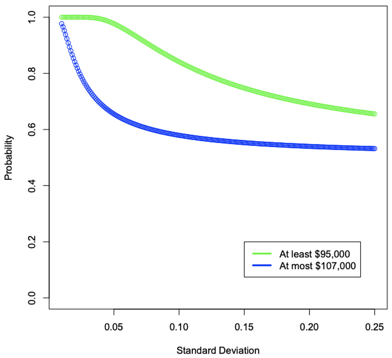

Please follow up with any feedback or doubts about this article, thanks.

~Roberto Baldizon