The Intuition behind the Z Transform

The Z transform plays a primordial role in signal and system analysis having a plethora of interesting applications in real life such as analysis and design of digital filters, automatic controllers, telecommunication systems, and much more. Every engineer, no matter his field of expertise, has come across the Z transform at one point or another during his college years. But what exactly is the intuition behind the Z transform and how does it correlate with the Laplace and the Fourier Transform?

Discrete-Time Signals and Systems

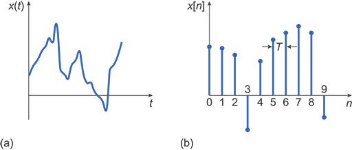
Unlike the Laplace and the Fourier Transforms which apply to continuous-time signals, the Z transforms is a discrete-time signal transform. Before we dive into the details of the Z transform, let’s take a moment to remind ourselves of the importance of discrete-time signals.

Of course, most quantities that we are interested in in real life are continuous quantities. Voltage, current, power, etc are all continuous quantities represented mathematically by continuous functions. In contrast, discrete-time signals are represented by sequences.

So why do we need discrete-time signals?

One of the most important and ground-breaking results in all of the information theory is the Sampling Theorem. Arguably, this theorem deserves an article on its own to fully understand it but we will briefly mention it here.

The Sampling Theorem establishes a sufficient condition for a sample rate that permits a discrete sequence of samples to capture all the information from a continuous-time signal of finite bandwidth.

In more simple terms, the Sampling theorem tells us that under certain simple conditions, we can capture all of the information of a continuous-time signal by a discrete sequence made up of a few of the original signal’s values. Sounds amazing right?

So, the sampling theorem allows to represent a continuous-time signal with a discrete-time one. This result is extremely important because discrete-time signals can be manipulated by systems instantiated as computer programs. Without the sampling theorem, we would have a really hard time using computers for any kind of signal processing.

In that sense, as counter-intuitive as it may sound, discrete-time signals are actually more general encompassing signals derived from continuous-time ones and signals that aren’t.

Without further ado, let’s now take a look at one of the main tools for processing discrete-time signals, the Z transform.

The Z Transform

The Z transform of a sequence x[n] is defined as follows.

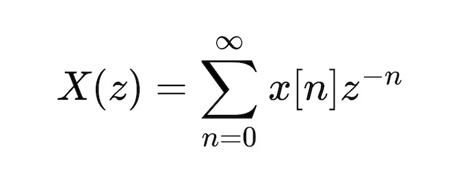
Again, as with every other transform found in signal analysis, we are transforming a function of time into a function of frequency.

Relation with the Laplace Transform

Let’s compare it side by side with the Laplace Transform so that we get a better understanding of its underlying mechanisms. Recall that the Laplace Transform (LT) of a function x(t) is given by the following integral.

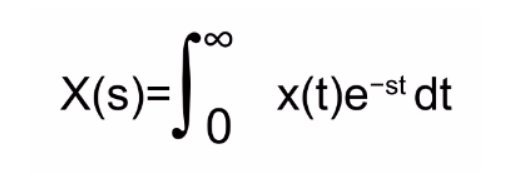
The first thing we notice is that in the case of the LT we have an integral while in the Z transform case we have a sum. This is to be expected since an integral is nothing but a limit of a sum as we transition from adding discrete quantities to continuous ones. Note that the limits of both the integral and the sum are the same (from 0 to positive infinity).

The main difference, however, is the presence of the “e” in the LT and its absence, correspondingly, in the Z transform sum.

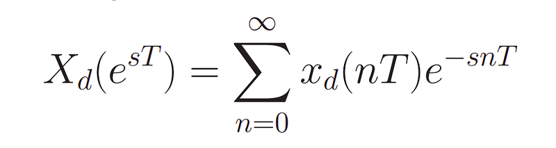
As we have already mentioned, most of the time, we are applying the Z transform to sequences that contain certain samples of a continuous-time signal. In this process of sampling we — usually — obtain these sample values with a period of T (every T units of time we get a value). Thus, if x = x(t) is the continuous-time signal, its sampled version can be expressed as x = x [nT].

We can now rewrite the aforementioned formula for the Z transform as follows:

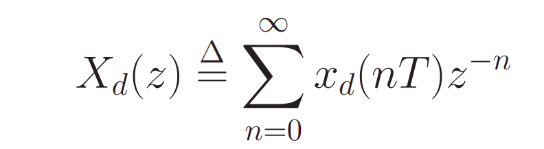
Let’s now give the following definition.

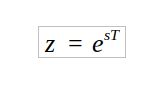
With this in mind, if we substitute z in the formula above we get:

If we now take the limit of the above quantity (times the sampling period/interval T) as the period T goes to zero (meaning that we get a continuous-time signal since we are sampling at infinitely small time intervals) we get:

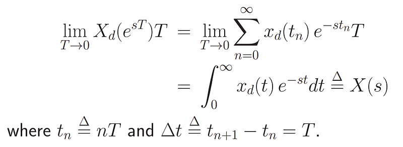
The Z transform is the discrete-time version of the Laplace Transform.

Mapping the s-plane into the z-plane and system stability

One of the most important properties of a system that the Laplace transform allows to analyze is its stability.

A control system is in equilibrium if, in the absence of any disturbance or input, the output stays in the same state.

A linear time-invariant control system is stable if the output eventually comes back to its equilibrium state when the system is subjected to an initial condition.

A linear time-invariant control system is critically stable if oscillations of the output continue forever.

It is unstable if the output diverges without bound from its equilibrium state when the system is subjected to an initial condition.

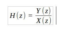
If x = x(t) is the input in our system and y = y(t) is our output then we define the Transfer function of the system as the ratio of the Laplace Transform of the output to the Laplace Transform of the input with all initial conditions being zero.

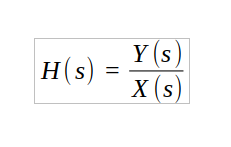
Lastly, the values of s that send H(s) to infinity i.e. the roots of its denominator are called the poles of the system.

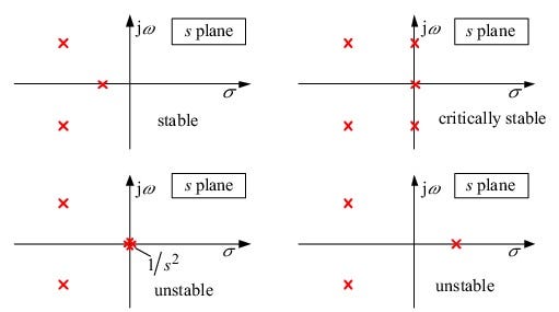
If all the poles of the Transfer function of a system are located in the left half of the s-plane then the system is stable. If there is at least one pole in the right half-plane and/or poles of multiplicity greater than 1 on the imaginary axis then the system is unstable. Finally, a system that has imaginary axis poles of multiplicity 1 yields pure sinusoidal oscillations as a natural response.

We see that the location of the poles completely defines a system’s stability. In the case of continuous time we can rely on the Laplace transform and the s-plane to provide us with that information.

But are the location requirements for a system to be stable in discrete time?

For this, we have to map the s-plane into the z-plane.

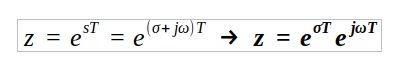
Remember how the z and s variables are related.

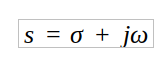
Both z and s are complex variables. We can write s as follows:

The relation above now becomes:

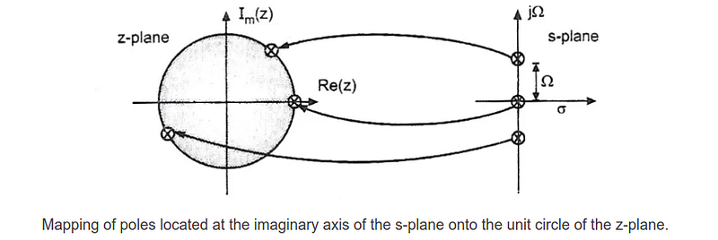
• If σ = 0 i.e. the s variable has no real part, then:

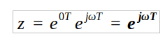
No matter the values of T and ω — as long as they are not 0 — then z will be located on the unit circle.

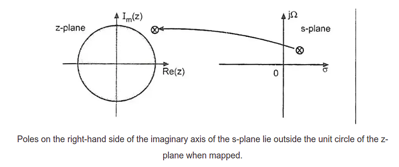
• If σ >0 i.e. the s variable has a positive real part, then:

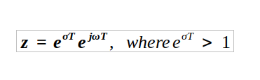
No matter the values of T and ω — as long as they are not 0 — then z will be located outside of the unit circle.

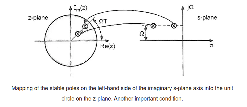
• If σ <0 i.e. the s variable has a negative real part, then:

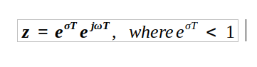
No matter the values of T and ω — as long as they are not 0 — then z will be located inside of the unit circle.

Final Remarks

You now know the basics of the Laplace transform. Obviously, we have only scratched the surface in this article but the intuition that you hopefully acquired from it will help you understand even more advanced concepts in engineering and physics in regards to the Laplace transform.

If you have any constructive criticism or any requests for a future “The Intuition behind…” article make sure to leave a comment or send me a message.

You can get full access to every story on Medium for just $5/month by signing up through this link.