The Input-Output Attention Mechanism from “Neural Machine Translation by Jointly Learning to Align and Translate”

The attention mechanism is an influential idea in deep learning. Even though we often think about attention as the one implemented in transformers, the original idea came from the paper “Neural Machine Translation by Jointly Learning to Align and Translate” by Dzmitry Bahdanau et. al.

Understanding the origin of this powerful attention technique helps us grasp many offspring ideas. In this article, I will describe this original attention idea. In future articles, I will cover other attentions, like the one from the Transformer model, and more recent ones not only on text, but also on images, videos and audios.

The language to language translation model

The paper introduced a model that translates one sentence from a source language into a sentence in a target language. The model has the encoder-decoder architecture where recursive neural network implements both the encoder and the decoder. The following chart shows the model architecture:

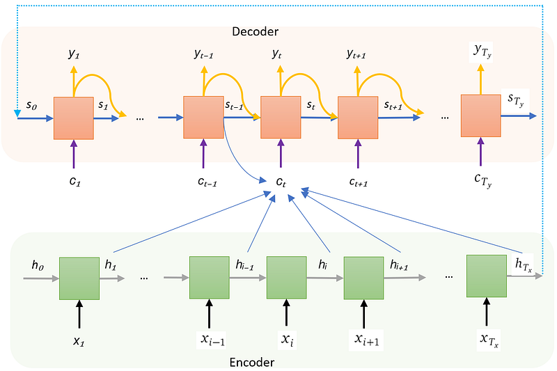
Model architecture

Let’s read the chart from bottom to top.

Inputs

At the bottom of the chart, inputs to the encoder is a sequence of words in the source language:

where

Tₓ is the length of the input sentence. For example, in a sentence “I love neural network”, Tₓ=4.
each xᵢ is a one-hot representation of a word in the source language with a dictionary of Kₓ words. That is, each xᵢ is a vector of length Kₓ, usually in the scale of 50 to 100 thousand words. Only one entry in this xᵢ vector is a one, indicating a particular word in the source language; all other entries are zero.

The encoder

The encoder is a recursive neural network. In the chart, it is shown as the usual consecutive blocks (the green ones). Remember, there is only one encoder block, all input words are processed by this block, one word after another.
An encoder block takes a hidden state and an input word, and emits the next hidden state. h₀, h₁…, h_Tₓ are hidden state vectors of length n. h₀ is a zero vector.
Note these encoder hidden state vectors are not model parameters, they are outputs from the recursive neural network block.
The last encoder hidden state h_Tₓ will be the initial state for the decoder, that is s_₀ = h_Tₓ. In the chart, the cyan dotted arrow establishes this connection.

The decoder

The decoder is also a recursive neural network, shown as pink blocks.
A decode block emits two things: the next translated word in the target language, and the next decoder hidden state. To do that, it takes three inputs: the previous decoder hidden state (shown as blue arrows), the previously outputted word (shown as yellow arrows), and a context (shown as purple arrow).
The context is the result from the attention mechanism and is the main purpose of this article. I will describe how to compute it and its intuition later.
The decoder continues to emit translated words until it emits a special end-of-sentence word.
Even though I drew the same amount of decoder blocks as the encoder blocks, during translation, the input and the outputted sentence are likely to be of different lengths.

More formally, the outputs from the decoder is a sequence of word probability vectors in the target language:

Tᵧ is the length of the target sentence, which we don’t know before the model finishes translating— we only know the target sentence length when the decoder outputs the special end-of-sentence word.
Each emitted probability vector yᵢ is of length Kᵧ, with Kᵧ being the dictionary size of the target language. The entries in the vector yᵢ are real numbers between 0 and 1, representing the probability of a particular word, i.e., the i-th word, where i is the entry index, in the target language. All the entries in yᵢ sums up to 1. The convention is to use the word with the highest probability as the i-th emitted word of the decoder.

Formulas

With the model architecture understood, let’s dive into the formulas that flow along the model, this helps us associate intuition to the corresponding mathematical implementations when we talk about the attention mechanism.

I simplified the formulas from the paper. My version of the formulas do not include bidirectional RNN, and LSTM style exponential smoothing. These simplification keeps the formulas short so it is easier to understand the main attention idea.

Encoder hidden state

Each encoder hidden state hᵢ is a vector of length n, with n being the dimension of the encoder hidden state. n is a hyper-parameter of the model, usually between hundreds and a few thousands.
The initial encoder hidden state is a zero vector. All consecutive encoder hidden states hᵢ is defined recursively by referencing the previous encoder hidden state hᵢ-₁. That’s the essence of recursive neural network.

Let’s look at the more interesting case of hᵢ. It combines information from the current input word xᵢ and the previous encoder hidden state hᵢ₋₁:

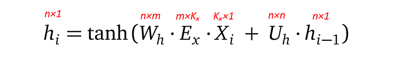
Xᵢ is the i-th input word in one-hot vector, with shape Kₓ×1.
Eₓ is the word embedding matrix for the source language, with shape m×Kₓ, with Kₓ being the number of words in the source language, and m being the dimension of the source language embedding.
hᵢ-₁ is the previous encoder hidden state.
Wₕ with shape n×m, and Uₕ with shape n×n are learnable parameters of the model.
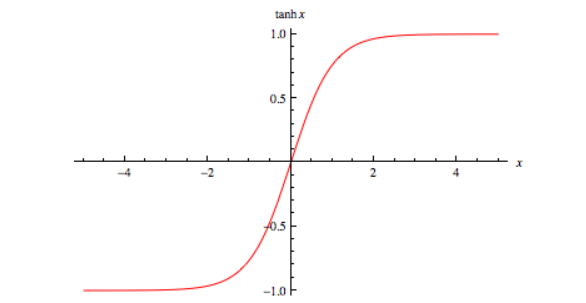
hyperbolic tangent tanh is the activation function. It squashes values from the full real domain into a range between -1 and 1.

I put the dimensions on top of various matrices so you can easily verify them.

The attention mechanism

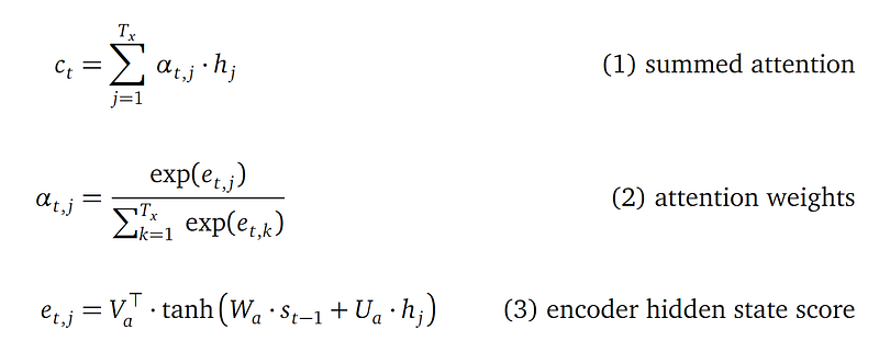
The attention mechanism computes a context vector for each output word. For the t-th output word, the context cₜ is a weighted average of all the encoder hidden states h₁ to h_Tx:

Or more concisely:

In the above formula, each αₜ,ⱼ is a float number, representing the weight to attend to the j-th input word’s hidden state hⱼ for the t-th output word. αₜ,ⱼ is defined using a softmax formula (the softmax function makes sure all the weights sum up to 1):

And eₜ,ⱼ is defined as:

eₜ,ⱼ combines information from the j-th encoder hidden state hⱼ and the (t-1)-th decoder hidden state sₜ₋₁.
Wₐ with shape n′×n and Uₐ with shape n′×n are learnable parameters.
Vₐ with shape n′×1 (so its transpose Vₐᵀ is of shape 1×n′) is also learnable parameter.
People refer to the expression at the righthand side of the above equation as the attention network because it is indeed a simple feedforward network. Let’s call it the attention score network.

Time complexity of the attention score network

Let’s think about how many times will the whole network, that is the encoder-decoder network, calls the attention score network to process a pair of input sentence of length Tₓ and target sentence of length Tᵧ. Here “process” means to feed the sentence pair into the whole network’s feed forward method.

For each word yₜ in the output sentence, the whole network needs to compute a context cₜ vector, so totally it computes Tᵧ number of context vectors.
To compute a single context vector cₜ, the whole network needs to feed forward the attention score network Tₓ number of times, with Tₓ being the input sentence length. This is because computing a context vector cₜ boils down to computing all the eₜ,ⱼvectors with j ranging over every word in the input sentence, so between [1, Tₓ].

So the whole network feeds forward the attention score network Tᵧ × Tₓ number of times. And this attention computation is sequential — first all the input words are processed by the encoder, and the output words by the decoder. This sequential nature causes the whole network to have a slow prediction time. This is solved in the “Attention is all you need” paper via the key, query and value design.

Intuition behind the attention mechanism

In a standard encoder-decoder architecture, information from the input sentence is only available to the decoder via the final encoder hidden state vector h_Tₓ, or equivalently, the initial decoder hidden state vector s_₀. This design:

Has the advantage of forcing the encoder to learn things about the input sentence. This is because the decoder can only rely on information from its initial hidden state vector to generate the output sentence. Only when the initial decoder hidden state vector contains enough information from the input sentence, the decide can do a good job in generating the output sentence.
The downside of this design is that when generating the output sentence, the decoder does not have access to specific input words, it only has information about the overall input sentence. Imagine that I ask you to translate a French novel (that’s our input sentence) into an English novel (that’s our output sentence), but I don’t give you the French novel, instead, I give you a summary of that novel (that’s the initial decoder hidden state vector), and require you to do a word-level translation. This is a hard task.

The motivation of the attention mechanism is to introduce a new way to pass information about the input words to the decoder. When setting up this new way, we need to think about the following:

When we reach the decoding stage, we’ve already have information for all the input words, stored in the encoder hidden states h₁, …, hⱼ, …, h_Tₓ.
The decoder generates, or decodes, the output sentence word by word: y₁, …, yₜ, … y_Ty.
Since not all input words are of equal importance when decoding an output word, when decoding the t-th output word, we need to decide which input words’ information, i.e., those encoder hidden state vectors, to pass to the decoder.

Given the above, the paper offers a clever design:

When decoding the t-th output words, instead of doing a binary decision on which input words to focus on, or attend to, the decoder includes information of all inputs words in a weighted sum way. That’s the cₜ vector.
The decoder then needs to learn how to assign weight to each input word when decoding the t-th output words. That’s the eₜ,ⱼ quantity, which is a float scalar value, for each of the j-th input words.

The eₜ,ⱼ quantity

The eₜ,ⱼ quantity ultimately decides how much information from an encoder hidden state hⱼ the model uses to decode an output word yₜ.

The larger an eₜ,ⱼ is, the higher the weight for the j-th encoder hidden state hⱼ (or equivalently the j-th input word), so more information from hⱼ is included in the computed context cₜ for decoding the t-th output word. The attention mechanism acts as a consultancy for the decoder. It tells the decoder, to generate the t-th output word, which input words to pay more attention to.

Now the question is how to compute eₜ,ⱼ? Alternatively, what information we use to compute eₜ,ⱼ? The above formula says to use the previous decoder hidden state sₜ₋₁ and the encoder hidden state hⱼ. This means:

we use information from the encoder hidden state for the j-th input word, that is hⱼ, which represents the knowledge about the input sentence “up to” the j-th word. Note the wording “up to”, because the hidden state hⱼ contains information from the first input word up to the j-th input word.
and we use information from the previous decoder hidden state sₜ₋₁, which represents the knowledge about the output sentence up to the t-th word.

These two pieces of information seems to be sensible choices. Are they the only choices? Maybe not. The authors of the paper decided on these choices and showed its experimental success. You can come up with other choices. In fact, in many followup attention ideas from other papers, you can see different choices.

The whole purpose of the attention mechanism is to compute the context vector to provide the decoder with better information from the input sentence. Now let’s see how the decode uses this context vector.

Decoder outputs

The decoder generates two outputs, the next decoder hidden state and the next output word in the target language.

Next decoder hidden state

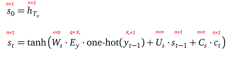
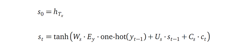
The first decode hidden state s_₀ is set to the last encoder hidden state h_Tx, that’s why s_₀ has the same shape as h_Tx, which is n×1.
All the consecutive decoder hidden states sₜ are defined recursively by referencing the previous decoder hidden state sₜ₋₁, among other things: the previously generated output word yₜ₋₁, the previous decoder state sₜ₋₁, and context cₜ from the attention mechanism. Please note the difference in the subscripts: sₜ₋₁, yₜ₋₁, but cₜ.
yₜ₋₁ is the output word probability vector (which is defined in the next section), whose length is Kᵧ. The one-hot operator turns yₜ₋₁ into a one-hot representation by assigning 1 to the vector entry with the largest value, and 0 to all other entries. This one-hot vector is used to select the embedding vector for that output word in the target language embedding matrix Eᵧ.
The target language embedding matrix Eᵧ is of shape q×Kᵧ, with Kᵧ being the number of words in the target language, and q being the dimension of the target language word embedding.
Wₛ, Uₛ and Cₛ are learnable parameters.

Next output word in the target language

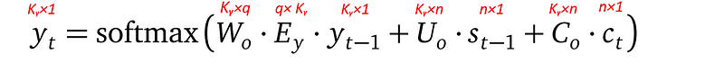
The output word probability vector yₜ combines three pieces of information: the previously generated output word yₜ₋₁, the previous decoder state sₜ₋₁, and context cₜ from the attention network. This is the same as the decoder hidden state sₜ.
But different matrices Wₒ, Uₒ and Cₒ (not Wₛ, Uₛ and Cₛ) are used to combine these pieces of information to generate yₜ, even though the structure of the combination formula is the same in yₜ as in sₜ.
Wₒ, Uₒ and Cₒ are learnable parameters.
The softmax operator makes sure that for an output word at position t, the probabilities of all words in the target language dictionary (whose size is size Kᵧ) sum up to 1.

This completes the language model that introduces the original attention mechanism.

Quick formula reference

I now lists all the formulas from above in a concise way for your quick reference:

(1) Encoder hidden state

(2) Attention network

(3) Decoder hidden state

(4) Target word probability vector from the decoder

Support me

If you like my story, I will be grateful if you consider supporting me by becoming a Medium member via this link: https://jasonweiyi.medium.com/membership.

I will keep writing these stories.

Conclusion

This article explains the recursive neural network based language to language translation model that introduced the attention mechanism for the first time. It clearly highlights how the input-output mechanism works and the intuition behind the math.