The importance and application of Vector Error Correction Model (VECM)

The auto regressive category has three distinct models; let is clear our understanding of them using the table below.

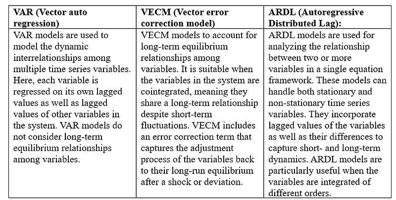
Each model has its own strengths and applicability depending on the characteristics of the data and the problem statement. VAR is suitable for short-term dynamics, VECM for long-term equilibrium relationships, and ARDL for analyzing relationships in a single equation framework with mixed-order integrated variables.

Here, we will discuss anout VECM and when do we apply error correctionj process. VECM is an extension of the Vector Autoregression (VAR) model where variables are assumed to be stationary. We can call VECM as cointegrated VAR. Wikipedia has a clear definition of error correction model. Many commonly used time series (for example, in economics) appear to be stationary in first differences. Forecasts from such a model will still reflect cycles and seasonality found in the data. However, any long-run changes that the data in levels may include are ignored, making longer-term estimates incorrect. This prompted Sargan to create “error correction model” to retain level information.

VECM is useful when dealing with economic and financial data where variables are often non-stationary and exhibit long-run relationships. .

Cointegration: When we have multiple time series variables that are non-stationary but are also cointegrated, meaning they share a long-term relationship despite potentially drifting apart in the short term.
Short- and Long-Run Dynamics: VECM allows us to model both the short-run dynamics (via lagged differences of the variables) and the long-run equilibrium relationships (via cointegrating vectors).
Granger Causality Tests: VECM can be used to investigate causal relationships among variables in both the short and long run, which is especially relevant in economic and financial analysis.
Error Correction Mechanism: VECM explicitly models the error correction term, which captures the short-term dynamics of how the variables adjust back to their long-run equilibrium after a shock.
Forecasting: VECM can be used for forecasting future values of the variables in the system, taking into account both short- and long-term relationships among them.

We selected two series in order to look for cointegration.

import yfinance as yf
import pandas as pd

_empty_series = pd.Series(dtype='float64')
sp_500 = yf.download('^GSPC', start='2020-01-01', end='2022-01-01')['Adj Close']
treasury_note_yield = yf.download('^TNX', start='2020-01-01', end='2022-01-01')['Adj Close']

import matplotlib.pyplot as plt

fig, axs = plt.subplots(1, 2, figsize=(15, 5))

# S&P 500
axs[0].plot(sp500)
axs[0].set_title('S&P 500')

# Treasury Note Yield
axs[1].plot(treasury_yield)
axs[1].set_title('Treasury Yield')

plt.tight_layout()
plt.show()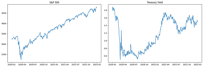

The non-stationarity shown in the above plots clearly indicates why this is a great candidate for VECM.

The Mathematics of Cointegration

Cointegration is a statistical concept that deals with the long-term equilibrium relationships among nonstationary time series. In the context of cointegration, we consider a group of time series yt, x1t and x2t. Here all these series are nonstationary. Cointegration means that even though these series are nonstationary, there exists a linear combination of them that is stationary which can be expressed: β1yt + β2x1t + β3x2t = et, here, et is the stationary series and linear combination of yt, x1t and x2t. β1, β2 and β3 are coefficients and are collectively known as the cointegrating vector. This vector determines how the cointegrating series are combined and normalized. Normalization of the cointegrating vector is necessary because there can be multiple vectors that fit the same economic model. A common normalization is to set β1=1, the equation becomes yt = -β2x1t — β3x2t — et. In the context of cointegration, normalization involves imposing restrictions on all the coefficients of the cointegrating relationship. In the example you provided, the normalization sets β1=1, which means we are normalizing one coefficient to a specific value. However, this does not mean that only one series is being normalized. It is a normalization choice to make the interpretation of the model more straightforward.

Johansen Cointegration test provides statistical evidence regarding the presence of cointegration relationships between the variables.

from statsmodels.tsa.vector_ar.vecm import coint_johansen

df = pd.concat([sp500, treasury_yield], axis=1)
df.columns = ['SP_500', 'treasury_note_yield']

specified_number = 0  # Testing for zero cointegrating relationships
coint_test_result = coint_johansen(df, specified_number, 1)

trace_stats = coint_test_result.lr2
eigen_stats = coint_test_result.lr1


print(f"Trace Statistics: {coint_test_result.lr1}")
print(f"Critical Values: {coint_test_result.cvt}")

# output
Trace Statistics: [11.24264977  0.01168631]
Critical Values: 
[[13.4294 15.4943 19.9349]
 [ 2.7055  3.8415  6.6349]]

The trace statistics represent the test statistics for the null hypothesis that the number of cointegrating relationships is less than or equal to the specified number (in this case, 0). Here, the trace statistics are [11.242 0.011] corresponding to the null hypothesis for 0 and 1 cointegrating relationships, respectively.

The critical values are thresholds against which the trace statistics are compared to determine statistical significance. They depend on the significance level (1%, 5%, or 10%) and the number of variables and observations in the dataset. Here, the first row [13.4294 15.4943 19.9349] corresponds to the critical values for the null hypothesis of 0 cointegrating relationships. The second row [ 2.7055 3.8415 6.6349] corresponds to the critical values for the null hypothesis of 1 cointegrating relationship.

For the trace statistic associated with the null hypothesis of 0 cointegrating relationships, we compare it with the critical values in the first row [13.4294 15.4943 19.9349]. Here, the trace statistic (11.042) is less than the critical values. If the trace statistics < than the critical values, it suggests that there is no evidence of cointegration among the variables. Thus, using VECM may not be appropriate. It indicates that the variables do not have a long-term equilibrium relationship that needs to be corrected for in the short run. A long-run equilibrium relationship means, both the series move together in such a way that their linear combination results in a stationary time series and they share an underlying common stochastic trend.

Here, VAR or ARIMA models may be appropriate.

# combining all
import yfinance as yf
import pandas as pd
from statsmodels.tsa.vector_ar.vecm import *

_empty_series = pd.Series(dtype='float64')

sp_500 = yf.download('^GSPC', start='2020-01-01', end='2022-01-01')['Adj Close']
treasury_note_yield = yf.download('^TNX', start='2020-01-01', end='2022-01-01')['Adj Close']

df = pd.concat([sp_500, treasury_note_yield], axis=1)
df.columns = ['sp500', 'treasury_note_yield']

cointegration_test_result = coint_johansen(df, det_order=0, k_ar_diff=1)

print("Johansen Cointegration Test Results:")
print(f"Trace Statistics: {cointegration_test_result.lr1}")
print(f"Critical Values: {cointegration_test_result.cvt}")

tracevalues = cointegration_test_result.lr1
critical_values = cointegration_test_result.cvt

data = [('sp500', 'treasury_note_yield')]

for i, (sp500, treasury_note_yield) in enumerate(data):
    if (tracevalues[i] > critical_values[:, 1]).all():
        print("\033[1msp500 and treasury_note_yield is cointegrated.\033[0m")
    else:
        print("\033[1msp500 and treasury_note_yield is not cointegrated.\033[0m")In practice, estimating the cointegration relationship separately before integrating it into the main model is a common approach.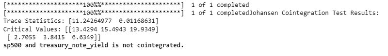

We further experimented with E-mini Russell 2000 Index Future (RTY=F) which brings a cointegrated series.

from matplotlib import pyplot as plt

russell_2000 = yf.download('RTY=F', start='2020-01-01', end='2022-01-01')['Adj Close']
treasury_note_yield = yf.download('^TNX', start='2020-01-01', end='2022-01-01')['Adj Close']

plt.figure()
ax = plt.subplot(211)
ax.plot(russell_2000)
ax.tick_params(axis='x', rotation=30)
ax = plt.subplot(212)
ax.plot(treasury_note_yield)
ax.tick_params(axis='x', rotation=30)
plt.tight_layout()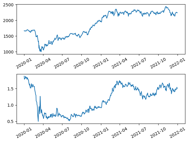

We notice from the plots that all observations are greater than zero, so we have a reason to include an intercept. Let us test the cointegration as shown below:

df = pd.concat([russell_2000, treasury_note_yield], axis=1)
df.columns = ['russell_2000', 'treasury_note_yield']

cointegration_test_result = coint_johansen(df, det_order=0, k_ar_diff=1)

print("Johansen Cointegration Test Results:")
print(f"Trace Statistics: {cointegration_test_result.lr1}")
print(f"Critical Values: {cointegration_test_result.cvt}")

tracevalues = cointegration_test_result.lr1
critical_values = cointegration_test_result.cvt

data = [('russell_2000', 'treasury_note_yield')]

for i, (russell_2000, treasury_note_yield) in enumerate(data):
    if (tracevalues[i] > critical_values[:, 1]).all():
        print("russell_2000_index and treasury_note_yield is cointegrated.")
    else:
        print("russell_2000_index and treasury_note_yield is not cointegrated.")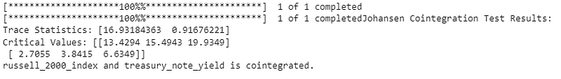

Here we see trace statistics > critical values indicating cointegrating relationships.

Short- and Long-Run Dynamics:

We can choose the lag order according to various information criteria (AIC, BIC, HQIC, and FPE).

from statsmodels.tsa.vector_ar import vecm

lagOrder = vecm.select_order(df, maxlags=15)
lagOrder.aic, lagOrder.bic, lagOrder.fpe, lagOrder.hqic

(9, 0, 9, 0)

We consider lag order 9 based on AIC (Akaike Information Criterion)

Cointegration rank

rank_test = select_coint_rank(df, 0, 9, method="trace", signif=0.05)
print(rank_test)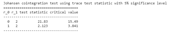

r_0 and r_1 are the hypothesized number of cointegrating vectors, which are the stationary linear combinations of the variables.
The test statistic is the value of the test statistic calculated from the data.
The critical value is the threshold value from the chi-squared distribution corresponding to the chosen significance level (5% in this case).

The last row contains the information about the cointegration rank to choose. Since the test statistic < critical value, we use r_0 as the cointegration rank. Otherwise we use r_1.

Mathematics of error correction

The error correction models provide a framework for analyzing the short-term dynamics of variables that are cointegrated, allowing researchers to study both the long-term equilibrium relationship and the short-term adjustment process between nonstationary series.

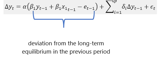
α is the speed of adjustment coefficient, indicating how quickly deviations from the long-term equilibrium are corrected.
δi are coefficients capturing the short-term dynamics of yt.
p is the order of the autoregressive component of the model. It indicates the number of lagged differences of the dependent variable included in the model to capture short-term dynamics and autocorrelation.
ϵt is the white noise error term.

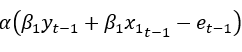
Above error correction term captures the short-term adjustment process whereby deviations from the long-term equilibrium are corrected. When the variables deviate from their long-term relationship, the error correction term will exert a force to bring them back towards equilibrium.

Parameter estimation

To fit a VECM to the data we build a VECM object where we define the deterministic terms, the lag order, and the cointegration rank.

russell_2000 = yf.download('RTY=F', start='2020-01-01', end='2022-01-01', interval='1d')['Adj Close'].values
treasury_note_yield = yf.download('^TNX', start='2020-01-01', end='2022-01-01', interval='1d')['Adj Close'].values

df = pd.DataFrame({'russell_2000': russell_2000, 'treasury_note_yield': treasury_note_yield})

model = VECM(df.values, deterministic="ci", 
             k_ar_diff=lagOrder.aic,  
             coint_rank=rankTest.rank)
result = model.fit()
result.summary()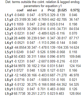

This output provides insights into the short-term dynamics (lagged parameters) and long-term equilibrium (cointegration relations) between the variables y1 and y2, as well as how they adjust to deviations from this equilibrium (error correction terms).

Equations for y1

Deterministic terms and lagged endogenous parameters:

The coefficients represent the effects of lagged values of both y1 and y2 on the current value of y1. L1.y1 represents the coefficient for the lagged value ofy1, and L1.y2 represents the coefficient for the lagged value of y2.

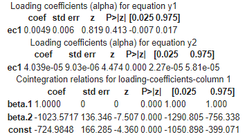
2. Loading coefficients for the error correction term:

The coefficient ec1 represents the loading coefficient for the error correction term ec1⋅Δy1.
This term captures the adjustment of y1 towards its long-run equilibrium relationship with y2.

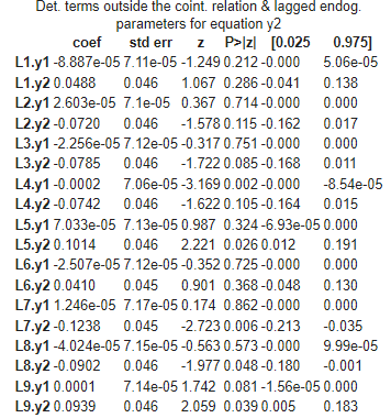
Equations for y2

Deterministic terms and lagged endogenous parameters:

Similar to the y1 equation, these coefficients represent the effects of lagged values of both y1 and y2 on the current value of y2.

2. Loading coefficients for the error correction term:

The coefficient ec1 represents the loading coefficient for the error correction term ec1⋅Δy2.
This term captures the adjustment of y2 towards its long-run equilibrium relationship with y1.

Cointegration relations

β1 represents the coefficient for the cointegrating vector corresponding to y1.
β2 represents the coefficient for the cointegrating vector corresponding to y2.
The constant term represents any intercept in the cointegration relationship.

Explanation

The loading coefficients for the error correction terms (ec1) indicate how each variable adjusts to deviations from its long-run equilibrium relationship with the other variable.
The cointegration relations (β1 and β2) show the long-term relationship between the variables y1 and y2, while the constant term represents any intercept in this relationship.

Hence, VECM provides estimates of short run behavior, long-run co-integrating relationship as well as short-run adjustment coefficients. The short run deviations from long-run equilibrium are corrected and the speed of this correction is shown by the adjustment coefficients as shown below.

error_correction_coef = result.alpha
print(error_correction_coef)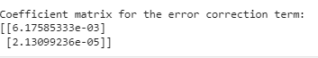

The first row corresponds to the russell_2000 variable. The second row corresponds to the Treasury Yield variable. Each column represents a lag of the error correction term. The coefficient for the error correction term for the variable russell_2000 is approximately 0.0062. The coefficient for the error correction term for the variable treasury_note_yield is approximately 0.0000213. These coefficients indicate the speed at which the variables adjust towards their long-run equilibrium in response to deviations from it. A larger coefficient indicates a faster adjustment process.

In practical terms, a positive coefficient indicates that there is a tendency for the variable to correct towards its long-run equilibrium level after a shock. A negative coefficient would suggest a tendency to move away from equilibrium, although this is less common.

Forecast

result.predict(steps=5, alpha=0.05)
for text, vaĺues in zip(("forecast", "lower", "upper"), result.predict(steps=5, alpha=0.05)):
    print(text+":", vaĺues, sep="\n")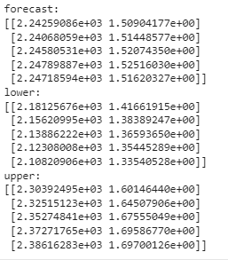

result.plot_forecast(steps=5, n_last_obs=12)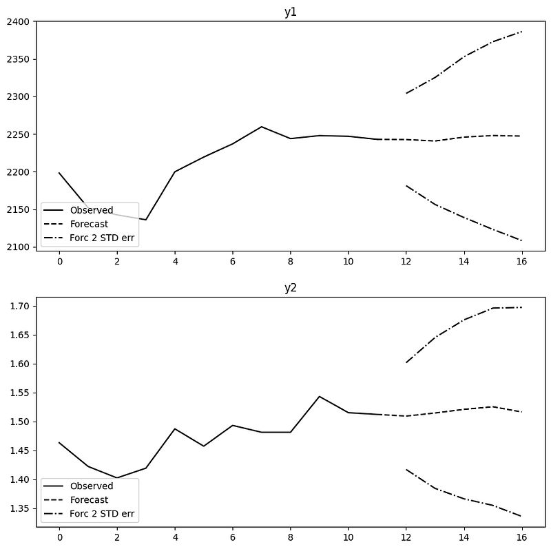

Here, we can opt for an alternative analysis using VAR (vector auto regression) and subsequently structural analysis using Granger Causality, Instantaneous causality, Impulse-Response-Analysis and more to diagnostics such as residual normality testing, checking residual autocorrelation using white test etc.

Key takeaways:

The Vector Error Correction Model (VECM) extends the VAR model to account for long-term equilibrium relationships among variables. It is suitable for cointegrated variables, implying a shared long-term relationship despite short-term fluctuations. The VECM model includes an error correction term that captures the adjustment process of variables back to their long-run equilibrium after a shock or deviation. The coefficients of the error correction term provide insights into the adjustment dynamics of each variable toward its long-run equilibrium relationship with other variables. VECM parameters are estimated using techniques like maximum likelihood estimation, and the model selection involves determining the appropriate lag order and cointegrating relationships. VECM analysis is valuable in various fields, including economics, finance, and environmental studies, where understanding long-term equilibrium relationships is crucial for decision-making and policy analysis.