The Hull Moving Average as a Trend Reversal Indicator

Presenting and Coding the Hull Moving Average in Time Series Analysis

The Hull Moving Average is a powerful trend-following overlay indicator that can be used to determine trends and capture them with less lag than the simple moving average. Its calculation is more complex but it is worth adding to the trading framework as it a confirmation factor. In this article, we will discuss the building blocks of the Hull Moving Average before coding and visualizing it.

Knowledge must be accessible to everyone. This is why, from now on, a purchase of either one of my new books “Contrarian Trading Strategies in Python” or “Trend Following Strategies in Python” comes with free PDF copies of my first three books (Therefore, purchasing one of the new books gets you 4 books in total). The two new books listed above feature a lot of advanced indicators and strategies with a GitHub page. You can use the below link to purchase one of the two books (Please specify which one and make sure to include your e-mail in the note).

The Concept of Moving Averages

Moving averages help us confirm and ride the trend. They are the most known technical indicator and this is because of their simplicity and their proven track record of adding value to the analyses. We can use them to find support and resistance levels, stops and targets, and to understand the underlying trend. This versatility makes them an indispensable tool in our trading arsenal.

As the name suggests, this is your plain simple mean that is used everywhere in statistics and basically any other part in our lives. It is simply the total values of the observations divided by the number of observations. Mathematically speaking, it can be written down as:

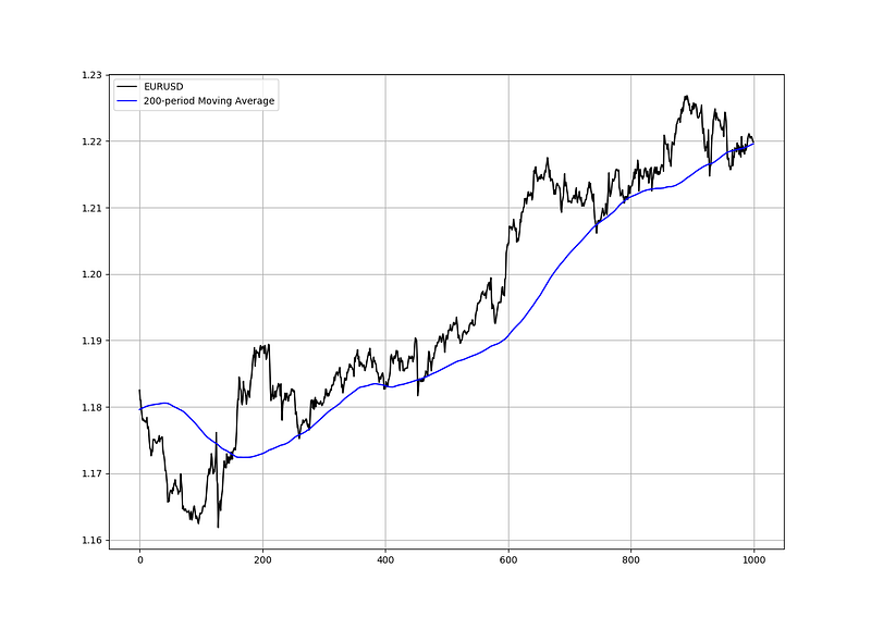
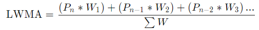
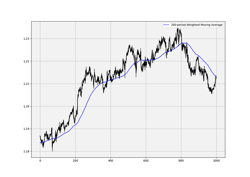
We can see that the moving average is providing decent dynamic support and resistance levels from where we can place our orders in case the market goes down there.

def ma(Data, lookback, what, where):
    
  for i in range(len(Data)):
      try:
        Data[i, where] = (Data[i - lookback + 1:i + 1, what].mean())
        
            except IndexError:
                pass
    return Data

Another even more dynamic moving average is the exponential one. Its idea is to give more weight to the more recent values so that it reduces the lag between the price and the average.

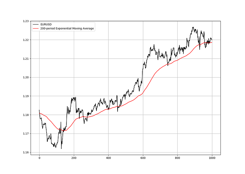
Notice how the exponential moving average is closer to prices than the simple one when the trend is strong. This is because it gives more weight to the latest values so that the average does not stay very far.

Let us now look at the first building block for the Hull Moving Average, i.e. the Weighted Moving Average.

Check out my weekly market sentiment report to understand the current positioning and to estimate the future direction of several major markets through complex and simple models working side by side. Find out more about the report through this link that covers the analysis between 07/08/2022 and 14/08/2022:

The Weighted Moving Average

Also referred to as a linear-weighted moving average, the weighted moving average is a simple moving average that places more weight on recent data. The most recent observation has the biggest weight and each one prior to it has a progressively decreasing weight. Intuitively, it has less lag than the other moving averages but it is also the least used, and hence, what it gains in lag reduction, it loses in popularity.

Mathematically speaking, it can be written down as:

Basically, if we have a dataset composed of two numbers [1, 2] and we want to calculate a linear weighted average, then we will do the following:

• (2 x 2) + (1 x 1) = 5
• 5 / 3 = 1.66

This assumes a time series with the number 2 as being the most recent observation.

import numpy as np

def lwma(Data, lookback):
    
    weighted = []
    for i in range(len(Data)):
            try:
                total = np.arange(1, lookback + 1, 1)
                
                matrix = Data[i - lookback + 1: i + 1, 3:4]
                matrix = np.ndarray.flatten(matrix)
                matrix = total * matrix
                wma = (matrix.sum()) / (total.sum())
                weighted = np.append(weighted, wma)

except ValueError:
                pass
    
    Data = Data[lookback - 1:, ]
    weighted = np.reshape(weighted, (-1, 1)) 
    Data = np.concatenate((Data, weighted), axis = 1)   
    
    return Data

# For this function to work, you need to have an OHLC array composed of the four usual columns, then you can use the below syntax to get a data array with the weighted moving average using the lookback you need

my_ohlc_data = lwma(my_ohlc_data, 20)

Now that we have understood what a Weighted Moving Average is, we can proceed by presenting the Hull Moving Average, a powerful trend-following early system.

The Hull Moving Average

The Hull Moving Average uses the Weighted Moving Average as building blocks and it is calculated following the below steps:

• Choose a lookback period such as 20 or 100 and calculate the Weighted Moving Average of the closing price.
• Divide the lookback period found in the first step and calculate the Weighted Moving Average of the closing price using this new lookback period. If the number cannot by divided by two, then take the closest number before the comma (e.g. a lookback of 15 can be 7 or 8 as the second lookback).
• Multiply the second Weighted Moving Average by two and subtract from it the first Weighted Moving Average.
• As a final step, take the square root of the first lookback (e.g. if you have chosen a lookback of 100, then the third lookback period is 10) and calculate the Weighted Moving Average on the latest result we have had in the third step. Be careful not to calculate it on market prices.

Therefore, if we choose a lookback period of 100, we will calculate on 100 lookback period, then on 50, and finally, on 10 applied to the latest result.

def adder(Data, times):
    
    for i in range(1, times + 1):
    
        z = np.zeros((len(Data), 1), dtype = float)
        Data = np.append(Data, z, axis = 1)

return Data

def hull_moving_average(Data, what, lookback, where):
    
    Data = lwma(Data, lookback, what)
    
    second_lookback = round((lookback / 2), 1)
    second_lookback = int(second_lookback) 
    
    Data = lwma(Data, second_lookback, what)
    
    Data = adder(Data, 1)
    Data[:, where + 2] = ((2 * Data[:, where + 1]) - Data[:, where])

third_lookback = round(np.sqrt(lookback), 1)
    third_lookback = int(third_lookback)

Data = lwma(Data, third_lookback, where + 2)

return Data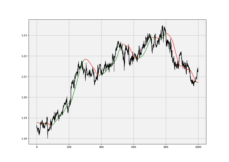

Why do we say that the Hull Moving Average reduces lag? The answer comes mainly from the building blocks which are the weighted moving averages. They place more weights on more recent values. Furthermore, the lag is also reduced by offsetting one weighted moving average with the one that has half the lookback period. Finally, we take the square root of the lookback period and apply it on the moving average itself using the weighting method. This gives us a moving average close to the market price and serves as an early trend reversal indicator.

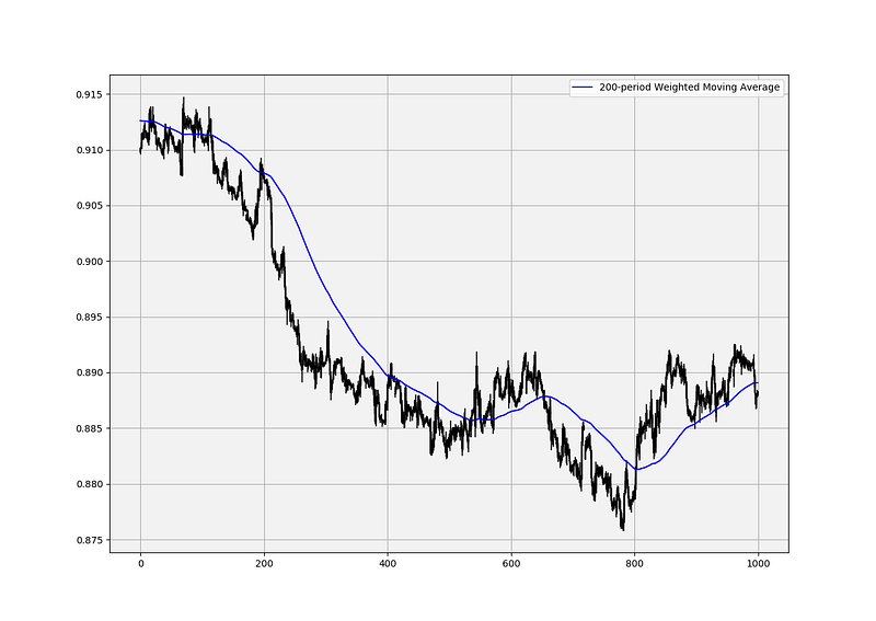
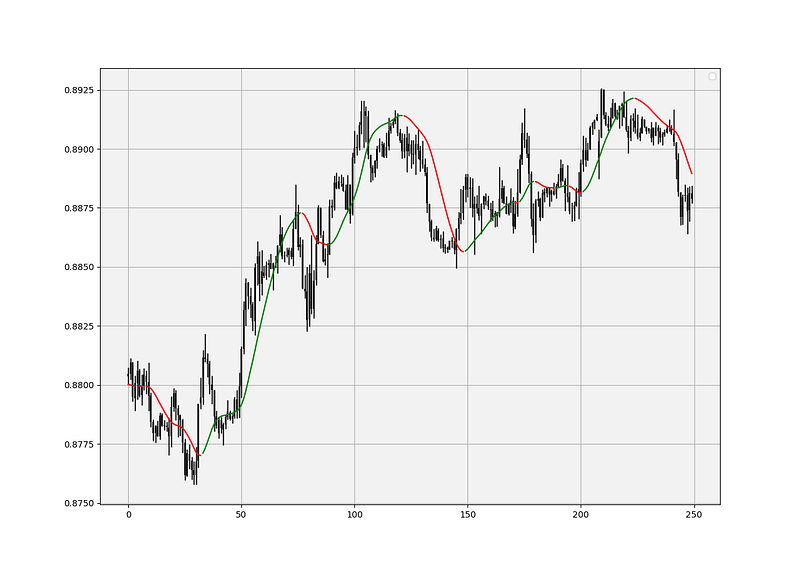
There is a special trick I like to use to add a visual component and helps to know whether the moving average is tilting to the upside or to the downside. Notice that in the chart above, when the moving average is pointing upwards, it is painted in green and when it is pointing downwards, it is painted in red. The way to do this is to simply put the following conditions:

• When the current moving average is greater than the one preceding it, then the next column should equal to the current moving average. Similarly, when the current moving average is less than the one preceding it, then the next column should equal to the current moving average divided by zero so that it gets an “inf” value in the array. This is so that when it is plotted on the chart, the “inf” values do not appear thus leaving the place for other values to be filled.
• When the current moving average is less than the one preceding it, then the next column should equal to the current moving average. Similarly, when the current moving average is greater than the one preceding it, then the next column should equal to the current moving average divided by zero so that it gets an “inf” value in the array.

The plotting function will be used on both new columns and we will choose our colors accordingly, giving us one moving average plot stemming from two columns, here is how to do this in Python:

my_data[:, new_column1] = my_data[:, hull_average]
my_data[:, new_column2] = my_data[:, hull_average]

for i in range(len(my_data)):
    if my_data[i, hull_average] > my_data[i - 1, hull_average]:
        my_data[i, new_column1] = my_data[i, hull_average]
        my_data[i, new_column2] = my_data[i, hull_average] / 0
        
    if my_data[i, hull_average] < my_data[i - 1, hull_average]:
        my_data[i, new_column2] = my_data[i, hull_average]  
        my_data[i, new_column1] = my_data[i, hull_average] / 0 
        
plt.plot(my_data[-1000:, new_column1], color = 'green')
plt.plot(my_data[-1000:, new_column2], color = 'red')

You can use this trick for pretty much any type of data.

Using the Hull Moving Average

The Hull Moving Average is used basically as you use any other moving average. However, I have a preference to use its slope as a signal rather than use it as a means to find support and resistance levels. Therefore, the difference (in my personal opinion) between the Hull Moving Average and the simple one is that the former is better in detecting early trend reversals but the latter is better used as support and resistance levels.

def signal(Data, what, buy, sell):
    
    for i in range(len(Data)):
            
        if Data[i, what] > Data[i - 1, what] and Data[i - 1, what] < Data[i - 2, what]:
            Data[i, buy] = 1
            
        if Data[i, what] < Data[i - 1, what] and Data[i - 1, what] > Data[i - 2, what]:
            Data[i, sell] = -1

# The what variable refers to the Hull Moving Average, and the buy and sell variables are the columns you want to put the long/short orders in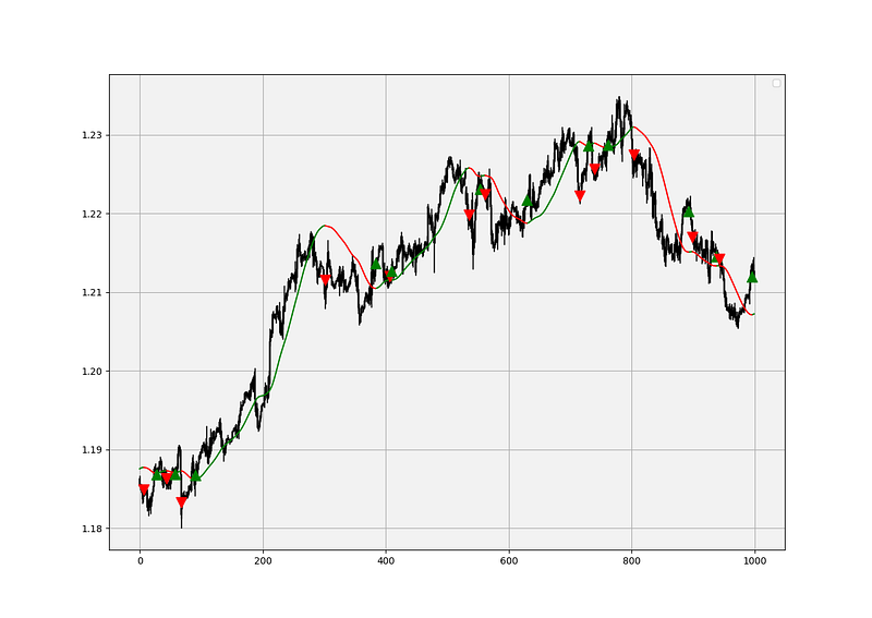

I am not a big fan of approaching zero lag as many indicators try to do. If you want to achieve zero lag, then all you need to do is to look at the price chart with no indicator overlaid on it. Some technical analysts claim to have zero lag moving averages which is very absurd because that means that the moving average would simply follow the price at every tick. How is that useful?

My preferred way of using moving averages is by simply confirming my support and resistance levels found through other ways.

If you want to see how to create all sorts of algorithms yourself, feel free to check out Lumiwealth. From algorithmic trading to blockchain and machine learning, they have hands-on detailed courses that I highly recommend.

Summary

To sum up, what I am trying to do is to simply contribute to the world of objective technical analysis which is promoting more transparent techniques and strategies that need to be back-tested before being implemented. This way, technical analysis will get rid of the bad reputation of being subjective and scientifically unfounded.

Medium is a hub to interesting reads. I read a lot of articles before I decided to start writing. Consider joining Medium using my referral link (at NO additional cost to you).

I recommend you always follow the the below steps whenever you come across a trading technique or strategy:

• Have a critical mindset and get rid of any emotions.
• Back-test it using real life simulation and conditions.
• If you find potential, try optimizing it and running a forward test.
• Always include transaction costs and any slippage simulation in your tests.
• Always include risk management and position sizing in your tests.

Finally, even after making sure of the above, stay careful and monitor the strategy because market dynamics may shift and make the strategy unprofitable.