The Hitchhiker’s Guide to Feature Extraction

Some Tricks and Code for Kaggle and Everyday work

Good Features are the backbone of any machine learning model.

And good feature creation often needs domain knowledge, creativity, and lots of time.

In this post, I am going to talk about:

Various methods of feature creation- Both Automated and manual
Different Ways to handle categorical features
Longitude and Latitude features
Some kaggle tricks
And some other ideas to think about feature creation.

TLDR; this post is about useful feature engineering methods and tricks that I have learned and end up using often.

1. Automatic Feature Creation using featuretools:

Have you read about featuretools yet? If not, then you are going to be delighted.

Featuretools is a framework to perform automated feature engineering. It excels at transforming temporal and relational datasets into feature matrices for machine learning.

How? Let us work with a toy example to show you the power of featuretools.

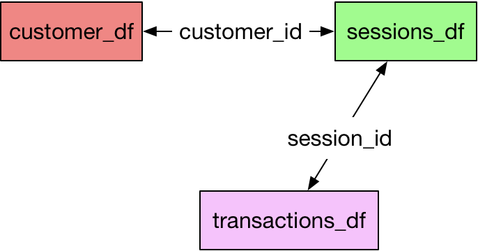
Let us say that we have three tables in our database: Customers, Sessions, and Transactions.

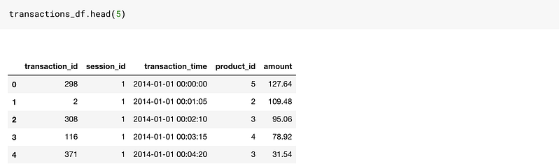
This is a reasonably good toy dataset to work on since it has time-based columns as well as categorical and numerical columns.

If we were to create features on this data, we would need to do a lot of merging and aggregations using Pandas.

Featuretools makes it so easy for us. Though there are a few things, we will need to learn before our life gets easier.

Featuretools works with entitysets.

You can understand an entityset as a bucket for dataframes as well as relationships between them.

Entityset = Bucket of dataframes and relationships

So without further ado, let us create an empty entityset. I just gave the name as customers. You can use any name here. It is just an empty bucket right now.

# Create new entityset
es = ft.EntitySet(id = 'customers')

Let us add our dataframes to it. The order of adding dataframes is not important. To add a dataframe to an existing entityset, we do the below operation.

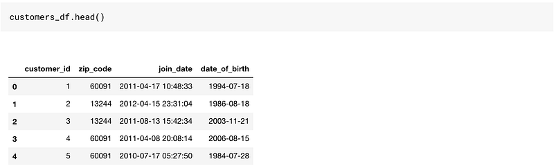
# Create an entity from the customers dataframe

es = es.entity_from_dataframe(entity_id = 'customers', dataframe = customers_df, index = 'customer_id', time_index = 'join_date' ,variable_types = {"zip_code": ft.variable_types.ZIPCode})

So here are a few things we did here to add our dataframe to the empty entityset bucket.

Provided a entity_id: This is just a name. Put it as customers.
dataframe name set as customers_df
index : This argument takes as input the primary key in the table
time_index : The time index is defined as the first time that any information from a row can be used. For customers, it is the joining date. For transactions, it will be the transaction time.
variable_types: This is used to specify if a particular variable must be handled differently. In our Dataframe, we have the zip_code variable, and we want to treat it differently, so we use this. These are the different variable types we could use:

[featuretools.variable_types.variable.Datetime,
 featuretools.variable_types.variable.Numeric,
 featuretools.variable_types.variable.Timedelta,
 featuretools.variable_types.variable.Categorical,
 featuretools.variable_types.variable.Text,
 featuretools.variable_types.variable.Ordinal,
 featuretools.variable_types.variable.Boolean,
 featuretools.variable_types.variable.LatLong,
 featuretools.variable_types.variable.ZIPCode,
 featuretools.variable_types.variable.IPAddress,
 featuretools.variable_types.variable.EmailAddress,
 featuretools.variable_types.variable.URL,
 featuretools.variable_types.variable.PhoneNumber,
 featuretools.variable_types.variable.DateOfBirth,
 featuretools.variable_types.variable.CountryCode,
 featuretools.variable_types.variable.SubRegionCode,
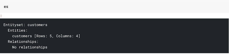
 featuretools.variable_types.variable.FilePath]

This is how our entityset bucket looks right now. It has just got one dataframe in it. And no relationships

Let us add all our dataframes:

# adding the transactions_df
es = es.entity_from_dataframe(entity_id="transactions",
                                 dataframe=transactions_df,
                                 index="transaction_id",
                               time_index="transaction_time",
                               variable_types={"product_id": ft.variable_types.Categorical})

# adding sessions_df
es = es.entity_from_dataframe(entity_id="sessions",
            dataframe=sessions_df,
            index="session_id", time_index = 'session_start')

This is how our entityset buckets look now.

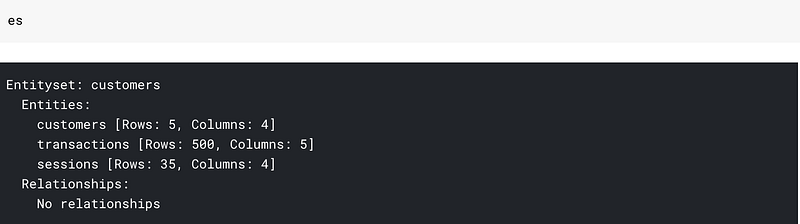
All three dataframes but no relationships. By relationships, I mean that my bucket doesn’t know that customer_id in customers_df and session_df are the same columns.

We can provide this information to our entityset as:

# adding the customer_id relationship
cust_relationship = ft.Relationship(es["customers"]["customer_id"],
                       es["sessions"]["customer_id"])

# Add the relationship to the entity set
es = es.add_relationship(cust_relationship)

# adding the session_id relationship
sess_relationship = ft.Relationship(es["sessions"]["session_id"],
                       es["transactions"]["session_id"])

# Add the relationship to the entity set
es = es.add_relationship(sess_relationship)

After this our entityset looks like:

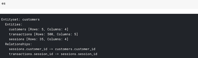
We can see the datasets as well as the relationships. Most of our work here is done. We are ready to cook features.

Cooking is no different from feature engineering. Think of features as ingredients.

Creating features is as simple as:

feature_matrix, feature_defs = ft.dfs(entityset=es, target_entity="customers",max_depth = 2)

feature_matrix.head()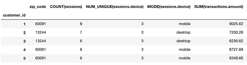

And we end up with 73 new features. You can see the feature names from feature_defs. Some of the features that we end up creating are:

[<Feature: NUM_UNIQUE(sessions.device)>,
 <Feature: MODE(sessions.device)>,
 <Feature: SUM(transactions.amount)>,
 <Feature: STD(transactions.amount)>,
 <Feature: MAX(transactions.amount)>,
 <Feature: SKEW(transactions.amount)>,
 <Feature: DAY(join_date)>,
 <Feature: YEAR(join_date)>,
 <Feature: MONTH(join_date)>,
 <Feature: WEEKDAY(join_date)>,
 <Feature: SUM(sessions.STD(transactions.amount))>,
 <Feature: SUM(sessions.MAX(transactions.amount))>,
 <Feature: SUM(sessions.SKEW(transactions.amount))>,
 <Feature: SUM(sessions.MIN(transactions.amount))>,
 <Feature: SUM(sessions.MEAN(transactions.amount))>,
 <Feature: SUM(sessions.NUM_UNIQUE(transactions.product_id))>,
 <Feature: STD(sessions.SUM(transactions.amount))>,
 <Feature: STD(sessions.MAX(transactions.amount))>,
 <Feature: STD(sessions.SKEW(transactions.amount))>,
 <Feature: STD(sessions.MIN(transactions.amount))>,
 <Feature: STD(sessions.MEAN(transactions.amount))>,
 <Feature: STD(sessions.COUNT(transactions))>,
 <Feature: STD(sessions.NUM_UNIQUE(transactions.product_id))>]

You can get features like the Sum of std of amount(SUM(sessions.STD(transactions.amount))) or std of the sum of amount(STD(sessions.SUM(transactions.amount))) This is what max_depth parameter means in the function call. Here we specify it as 2 to get two level aggregations.

If we change max_depth to 3 we can get features like: MAX(sessions.NUM_UNIQUE(transactions.YEAR(transaction_time)))

Just think of how much time you would have to spend if you had to write code to get such features. Also, a caveat is that increasing the max_depth might take longer times.

2. Handling Categorical Features: Label/Binary/Hashing and Target/Mean Encoding

Creating automated features has its perks. But why would we data scientists be required if a simple library could do all our work?

This is the section where I will talk about handling categorical features.

One hot encoding

We can use One hot encoding to encode our categorical features. So if we have n levels in a category, we will get n-1 features.

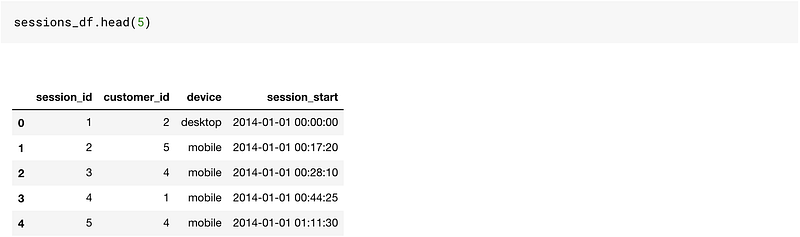
In our sessions_df table, we have a column named device, which contains three levels — desktop, mobile, or tablet. We can get two columns from such a column using:

pd.get_dummies(sessions_df['device'],drop_first=True)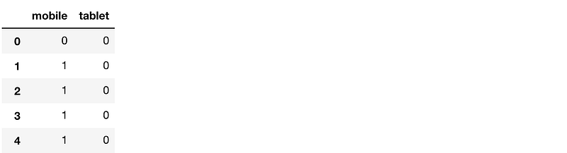

This is the most natural thing that comes to mind when talking about categorical features and works well in many cases.

OrdinalEncoding

Sometimes there is an order associated with categories. In such a case, I usually use a simple map/apply function in pandas to create a new ordinal column.

For example, if I had a dataframe containing temperature as three levels: high medium and low, I would encode that as:

map_dict = {'low':0,'medium':1,'high':2}
def map_values(x):
    return map_dict[x]
df['Temperature_oe'] = df['Temperature'].apply(lambda x: map_values(x))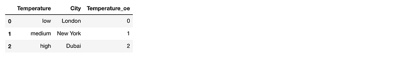

Using this I preserve the information that low

LabelEncoder

We could also have used LabelEncoder to encode our variable to numbers. What a label encoder essentially does is that it sees the first value in the column and converts it to 0, next value to 1 and so on. This approach works reasonably well with tree models, and I end up using it when I have a lot of levels in the categorical variable. We can use this as:

from sklearn.preprocessing import LabelEncoder
# create a labelencoder object
le = LabelEncoder()
# fit and transform on the data
sessions_df['device_le'] = le.fit_transform(sessions_df['device'])
sessions_df.head()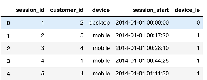

BinaryEncoder

BinaryEncoder is another method that one can use to encode categorical variables. It is an excellent method to use if you have many levels in a column. While we can encode a column with 1024 levels using 1023 columns using One Hot Encoding, using Binary encoding we can do it by just using ten columns.

Let us say we have a column in our FIFA 19 player data that contains all club names. This column has 652 unique values. One Hot encoding means creating 651 columns that would mean a lot of memory usage and a lot of sparse columns.

If we use Binary encoder, we will only need ten columns as 2⁹<652 <2¹⁰.

We can binaryEncode this variable easily by using BinaryEncoder object from category_encoders:

from category_encoders.binary import BinaryEncoder
# create a Binaryencoder object
be = BinaryEncoder(cols = ['Club'])
# fit and transform on the data
players = be.fit_transform(players)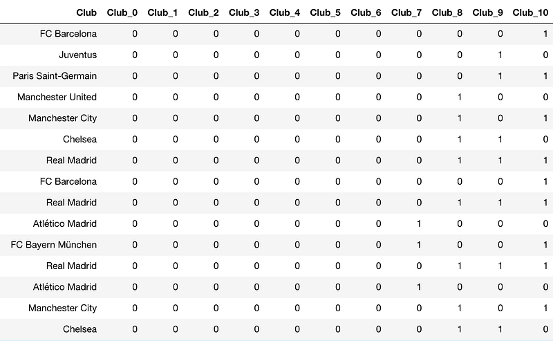

HashingEncoder

One can think of Hashing Encoder as a black box function that converts a string to a number between 0 to some prespecified value.

It differs from binary encoding as in binary encoding two or more of the club parameters could have been 1 while in hashing only one value is 1.

We can use hashing as:

players = pd.read_csv("../input/fifa19/data.csv")

from category_encoders.hashing import HashingEncoder
# create a HashingEncoder object
he = HashingEncoder(cols = ['Club'])
# fit and transform on the data
players = he.fit_transform(players)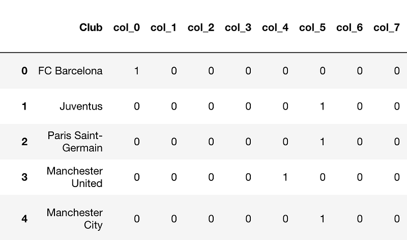

There are bound to be collisions(two clubs having the same encoding. For example, Juventus and PSG have the same encoding) but sometimes this technique works well.

Target/Mean Encoding

This is a technique that I found works pretty well in Kaggle competitions. If both training/test comes from the same dataset from the same time period(cross-sectional), we can get crafty with features.

For example: In the Titanic knowledge challenge, the test data is randomly sampled from the train data. In this case, we can use the target variable averaged over different categorical variable as a feature.

In Titanic, we can create a target encoded feature over the PassengerClass variable.

We have to be careful when using Target encoding as it might induce overfitting in our models. Thus we use k-fold target encoding when we use it.

We can then create a mean encoded feature as:

targetc = KFoldTargetEncoderTrain('Pclass','Survived',n_fold=5)
new_train = targetc.fit_transform(train)

new_train[['Pclass_Kfold_Target_Enc','Pclass']]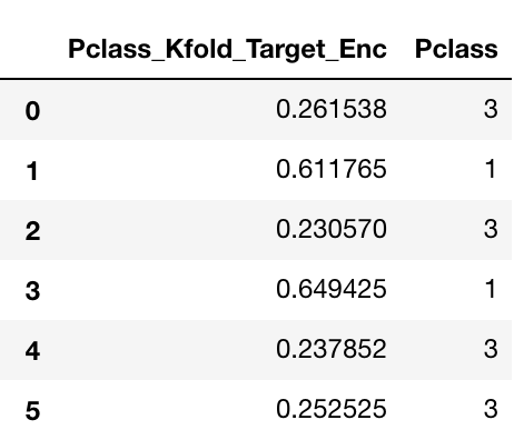

You can see how the passenger class 3 gets encoded as 0.261538 and 0.230570 based on which fold the average is taken from.

This feature is pretty helpful as it encodes the value of the target for the category. Just looking at this feature, we can say that the Passenger in class 1 has a high propensity of surviving compared with Class 3.

3. Some Kaggle Tricks:

While not necessarily feature creation techniques, some postprocessing techniques that you may find useful.

log loss clipping Technique:

Something that I learned in the Neural Network course by Jeremy Howard. It is based on an elementary Idea.

Log loss penalizes us a lot if we are very confident and wrong.

So in the case of Classification problems where we have to predict probabilities in Kaggle, it would be much better to clip our probabilities between 0.05–0.95 so that we are never very sure about our prediction. And in turn, get penalized less. Can be done by a simple np.clip

Kaggle submission in gzip format:

A small piece of code that will help you save countless hours of uploading. Enjoy.

df.to_csv(‘submission.csv.gz’, index=False, compression=’gzip’)

4. Using Latitude and Longitude features:

This part will tread upon how to use Latitude and Longitude features well.

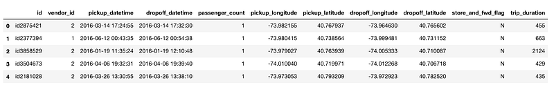
For this task, I will be using Data from the Playground competition: New York City Taxi Trip Duration

The train data looks like:

Most of the functions I am going to write here are inspired by a Kernel on Kaggle written by Beluga.

In this competition, we had to predict the trip duration. We were given many features in which Latitude and Longitude of pickup and Dropoff were also there. We created features like:

A. Haversine Distance Between the Two Lat/Lons:

The haversine formula determines the great-circle distance between two points on a sphere given their longitudes and latitudes

def haversine_array(lat1, lng1, lat2, lng2): 
    lat1, lng1, lat2, lng2 = map(np.radians, (lat1, lng1, lat2, lng2)) 
    AVG_EARTH_RADIUS = 6371 # in km 
    lat = lat2 - lat1 
    lng = lng2 - lng1 
    d = np.sin(lat * 0.5) ** 2 + np.cos(lat1) * np.cos(lat2) *      np.sin(lng * 0.5) ** 2 
    h = 2 * AVG_EARTH_RADIUS * np.arcsin(np.sqrt(d)) 
    return h

We could then use the function as:

train['haversine_distance'] = train.apply(lambda x: haversine_array(x['pickup_latitude'], x['pickup_longitude'], x['dropoff_latitude'], x['dropoff_longitude']),axis=1)

B. Manhattan Distance Between the two Lat/Lons:

The distance between two points measured along axes at right angles

def dummy_manhattan_distance(lat1, lng1, lat2, lng2): 
    a = haversine_array(lat1, lng1, lat1, lng2) 
    b = haversine_array(lat1, lng1, lat2, lng1) 
    return a + b

We could then use the function as:

train['manhattan_distance'] = train.apply(lambda x: dummy_manhattan_distance(x['pickup_latitude'], x['pickup_longitude'], x['dropoff_latitude'], x['dropoff_longitude']),axis=1)

C. Bearing Between the two Lat/Lons:

A bearing is used to represent the direction of one point relative to another point.

def bearing_array(lat1, lng1, lat2, lng2): 
    AVG_EARTH_RADIUS = 6371 # in km 
    lng_delta_rad = np.radians(lng2 - lng1) 
    lat1, lng1, lat2, lng2 = map(np.radians, (lat1, lng1, lat2, lng2)) 
    y = np.sin(lng_delta_rad) * np.cos(lat2) 
    x = np.cos(lat1) * np.sin(lat2) - np.sin(lat1) * np.cos(lat2) * np.cos(lng_delta_rad) 
    return np.degrees(np.arctan2(y, x))

We could then use the function as:

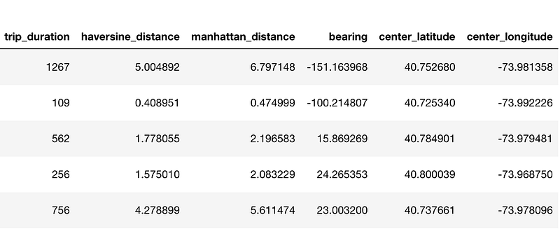
train['bearing'] = train.apply(lambda x: bearing_array(x['pickup_latitude'], x['pickup_longitude'], x['dropoff_latitude'], x['dropoff_longitude']),axis=1)

D. Center Latitude and Longitude between Pickup and Dropoff:

train.loc[:, 'center_latitude'] = (train['pickup_latitude'].values + train['dropoff_latitude'].values) / 2 
train.loc[:, 'center_longitude'] = (train['pickup_longitude'].values + train['dropoff_longitude'].values) / 2

These are the new columns that we create:

5. AutoEncoders:

Sometimes people use Autoencoders too for creating automatic features.

What are Autoencoders?

Encoders are deep learning functions which approximate a mapping from X to X, i.e. input=output. They first compress the input features into a lower-dimensional representation and then reconstruct the output from this representation.

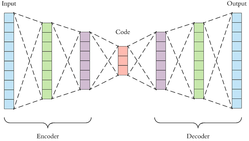
We can use this representation vector as a feature for our models.

6. Some Normal Things you can do with your features:

Scaling by Max-Min: This is good and often required preprocessing for Linear models, Neural Networks
Normalization using Standard Deviation: This is good and often required preprocessing for Linear models, Neural Networks
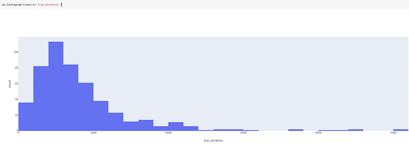
Log-based feature/Target: Use log based features or log-based target function. If one is using a Linear model which assumes that the features are normally distributed, a log transformation could make the feature normal. It is also handy in case of skewed variables like income.

Or in our case trip duration. Below is the graph of trip duration without log transformation.

And with log transformation:

train['log_trip_duration'] = train['trip_duration'].apply(lambda x: np.log(1+x))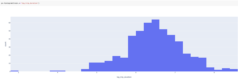

A log transformation on trip duration is much less skewed and thus much more helpful for a model.

7. Some Additional Features based on Intuition:

Date time Features:

One could create additional Date time features based on domain knowledge and intuition. For example, Time-based Features like “Evening,” “Noon,” “Night,” “Purchases_last_month,” “Purchases_last_week,” etc. could work for a particular application.

Domain-Specific Features:

Suppose you have got some shopping cart data and you want to categorize the TripType. It was the exact problem in Walmart Recruiting: Trip Type Classification on Kaggle.

Some examples of trip types: a customer may make a small daily dinner trip, a weekly large grocery trip, a trip to buy gifts for an upcoming holiday, or a seasonal trip to buy clothes.

To solve this problem, you could think of creating a feature like “Stylish” where you create this variable by adding together the number of items that belong to category Men’s Fashion, Women’s Fashion, Teens Fashion.

Or you could create a feature like “Rare” which is created by tagging some items as rare, based on the data we have and then counting the number of those rare items in the shopping cart.

Such features might work or might not work. From what I have observed, they usually provide a lot of value.

I feel this is the way that Target’s “Pregnant Teen model” was made. They would have had a variable in which they kept all the items that a pregnant teen could buy and put them into a classification algorithm.

Interaction Features:

If you have features A and B, you can create features A*B, A+B, A/B, A-B, etc.

For example, to predict the price of a house, if we have two features length and breadth, a better idea would be to create an area(length x breadth) feature.

Or in some case, a ratio might be more valuable than having two features alone. Example: Credit Card utilization ratio is more valuable than having the Credit limit and limit utilized variables.

Conclusion

These were just some of the methods I use for creating features.

But there is surely no limit when it comes to feature engineering, and it is only your imagination that limits you.

On that note, I always think about feature engineering while keeping what model I am going to use in mind. Features that work in a random forest may not work well with Logistic Regression.

Feature creation is the territory of trial and error. You won’t be able to know what transformation works or what encoding works best before trying it. It is always a trade-off between time and utility.

Sometimes the feature creation process might take a lot of time. In such cases, you might want to parallelize your Pandas function.

While I have tried to keep this post as exhaustive as possible(This might very well be my biggest post on medium yet), I might have missed some of the useful methods. Let me know about them in the comments.

You can find all the code for this post and run it yourself in this Kaggle Kernel

Take a look at the Advanced Machine Learning on Google Cloud Specialization. This course talks about deploy and productionizing your models. Definitely recommended.

I am going to be writing more beginner friendly posts in the future too. Let me know what you think about the series. Follow me up at Medium or Subscribe to my blog to be informed about them. As always, I welcome feedback and constructive criticism and can be reached on Twitter @mlwhiz.