CAUSAL DATA SCIENCE

Understanding the Frisch-Waugh-Lovell Theorem

A step-by-step guide to one of the most powerful theorems in causal inference

The Frisch-Waugh-Lowell theorem is a simple yet powerful theorem that allows us to reduce multivariate regressions to univariate ones. This is extremely useful when we are interested in the relationship between two variables, but we still need to control for other factors, as is often the case in causal inference.

In this blog post, I am going to introduce the Frisch-Waugh-Lowell theorem and illustrate some interesting applications.

The Theorem

The theorem was first published by Ragnar Frisch and Frederick Waugh in 1933. However, since its proof was lengthy and cumbersome, Michael Lovell in 1963 provided a straightforward and intuitive proof and his name was added to the theorem name.

The theorem states that when estimating a model of the form

then, the following estimators of β₁ are equivalent:

the OLS estimator obtained by regressing y on x₁ and x₂
the OLS estimator obtained by regressing y on x̃₁, where x̃₁ is the residual from the regression of x₁ on x₂
the OLS estimator obtained by regressing ỹ on x̃₁, where ỹ is the residual from the regression of y on x₂

Interpretation

What did we actually learn from it?

The Frisch-Waugh-Lowell theorem is telling us that there are multiple ways to estimate a single regression coefficient. One possibility is to run the full regression of y on x, as usual.

However, we can also regress x₁ on x₂, take the residuals, and regress y only those residuals. The first part of this process is sometimes referred to as partialling-out (or orthogonalization, or residualization) of x₁ with respect to x₂. The idea is that we are isolating the variation in x₁ that is orthogonal to x₂. Note that x₂ can also be multi-dimensional (i.e. include multiple variables and not just one).

Why would one ever do that?

This seems like a way more complicated procedure. Instead of simply doing the regression in 1 step, now we need to do 2 or even 3 steps. It’s not intuitive at all. The main advantage comes from the fact that we have reduced a multivariate regression to a univariate one, making it more tractable and more intuitive.

We will later explore more in detail three applications:

data visualization
computational speed
further applications for inference

However, let’s first explore the theorem more in detail with an example.

Example

Suppose we were a retail chain, owning many different stores in different locations. We come up with a brilliant idea to increase sales: give away discounts in the form of coupons. We print a lot of coupons and we distribute them around.

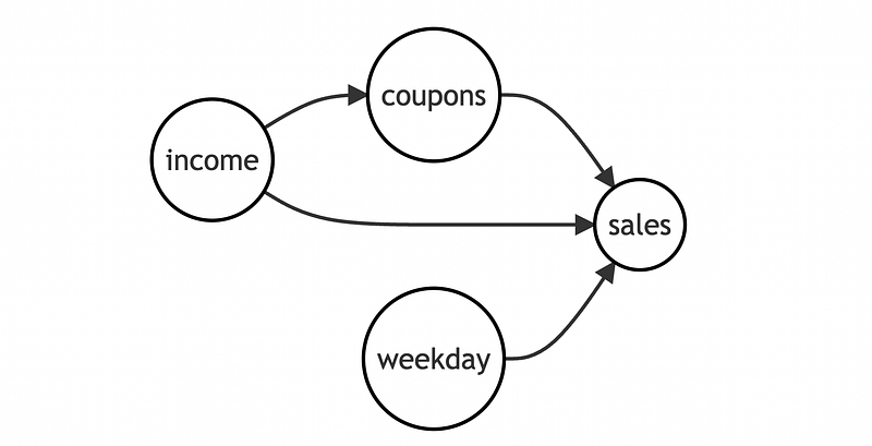
To understand whether our marketing strategy worked, in each store, we check the average daily sales and which percentage of shoppers used a coupon. However, there is one problem: we are worried that higher income people are less likely to use the discount, but usually they spend more. To be safe, we also record the average income in the neighborhood of each store.

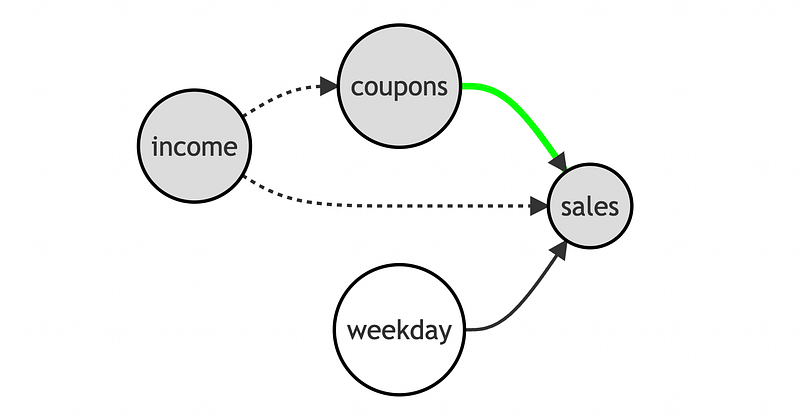
We can represent the data generating process with a Directed Acyclic Graph (DAG). If you are not familiar with DAGs, I have written a short introduction to Directed Acyclic Graphs here.

Let’s load and inspect the data. I import the data generating process from src.dgp and some plotting functions and libraries from src.utils.

from src.utils import *
from src.dgp import dgp_store_coupons

df = dgp_store_coupons().generate_data(N=50)
df.head()

We have information on 50 stores, for which we observe the percentage of customers that use coupons, daily sales (in thousand $), average income of the neighborhood (in thousand $), and day of the week.

Suppose we were directly regressing sales on coupon usage. What would we get? I represent the result of the regression graphically, using seaborn regplot.

import seaborn as sns

sns.regplot(x="coupons", y="sales", data=df, ci=False, line_kws={'color':'r', 'label':'linear fit'})
plt.legend()
plt.title(f"Sales and coupon usage");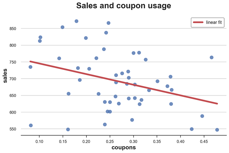

It looks like coupons were a bad idea: in stores where coupons are used more, we observe lower sales.

However, it might just be that people with higher income are using fewer coupons, while also spending more. If this was true, it could bias our results. In terms of the DAG, it means that we have a backdoor path passing through income, generating a non-causal relationship.

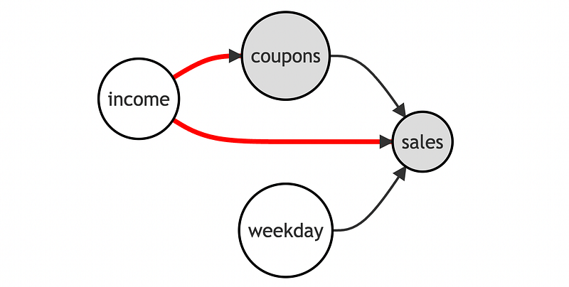
In order to recover the causal effect of coupons on sales we need to condition our analysis on income. This will block the non-causal path passing through income, leaving only the direct path from coupons to sales open, allowing us to estimate the causal effect.

Let’s implement this, by including income in the regression.

import statsmodels.formula.api as smf

smf.ols('sales ~ coupons + income', df).fit().summary().tables[1]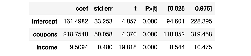

Now the estimated effect of coupons on sales is positive and significant. Coupons were a good idea after all.

Verifying the Theorem

Let’s now verify that the Frisch-Waugh-Lowell theorem actually holds. In particular, we want to check whether we get the same coefficient if, instead of regressing sales on coupons and income, we were

regressing coupons on income
computing the residuals coupons_tilde, i.e. the variation in coupons not explained by income
regressing sales on coupons_tilde

Note that I add “-1” to the regression formula to remove the intercept.

df['coupons_tilde'] = smf.ols('coupons ~ income', df).fit().resid

smf.ols('sales ~ coupons_tilde - 1', df).fit().summary().tables[1]

Now the coefficient is the same! However, the standard errors have increased a lot and the estimated coefficient is not significantly different from zero anymore.

A better approach is to add a further step and repeat the same procedure also for sales:

regress sales on income
compute the residuals sales_tilde, i.e. the variation in sales not explained by income
finally, regress sales_tilde on coupons_tilde

df['sales_tilde'] = smf.ols('sales ~ income', df).fit().resid

smf.ols('sales_tilde ~ coupons_tilde - 1', df).fit().summary().tables[1]

The coefficient is still exactly the same, but now also the standard errors are almost identical.

Projection

What is partialling-out (or residualization, or orthogonalization) actually doing? What is happening when we take the residuals of coupons with respect to income?

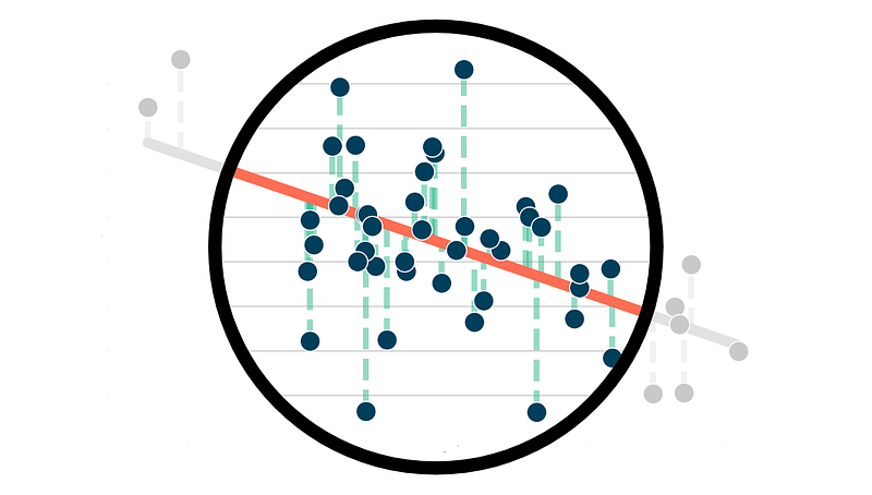
We can visualize the procedure in a plot. First, let’s display the residuals of coupons with respect to income.

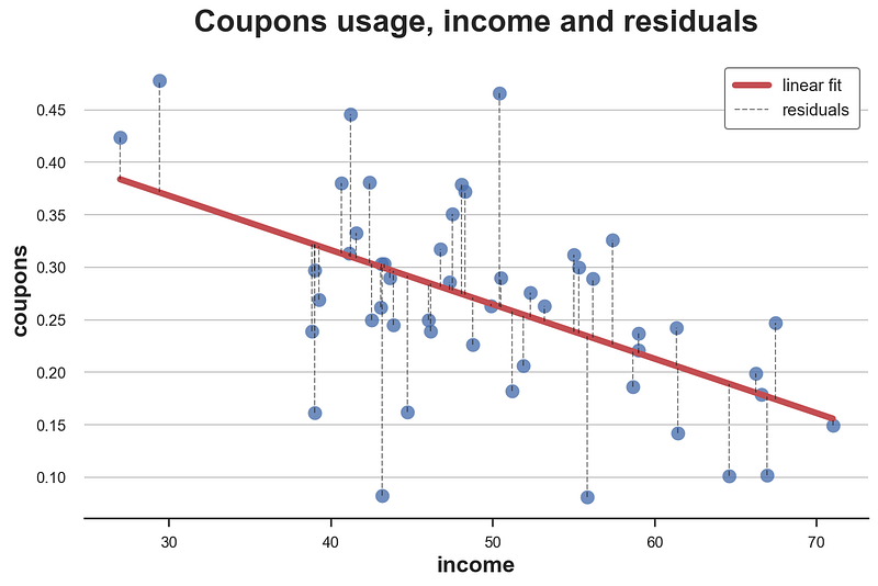
The residuals are the vertical dotted lines between the data and the linear fit, i.e. the part of the variation in coupons unexplained by income.

By partialling-out, we are removing the linear fit from the data and keeping only the residuals. We can visualize this procedure with a gif. I import the code from the src.figures file that you can find here.

from src.figures import gif_projection

gif_projection(x='income', y='coupons', df=df, gifname="gifs/fwl.gif")

The original distribution of the data is on the left in blue, and the partialled-out data is on the right in green. As we can see, partialling-out removes both the level and the trend in coupons that is explained by income.

Multiple Controls

We can use the Frisch-Waugh-Theorem also when we have multiple control variables. Suppose that we also wanted to include day of the week in the regression, to increase precision.

smf.ols('sales ~ coupons + income + dayofweek', df).fit().summary().tables[1]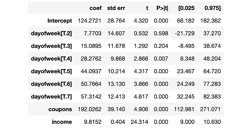

We can perform the same procedure as before, but instead of partialling-out only income, now we partial out both income and day of the week.

df['coupons_tilde'] = smf.ols('coupons ~ income + dayofweek', df).fit().resid
df['sales_tilde'] = smf.ols('sales ~ income + dayofweek', df).fit().resid

smf.ols('sales_tilde ~ coupons_tilde - 1', df).fit().summary().tables[1]

We still get exactly the same coefficient!

Applications

Let’s now inspect some applications of the FWL theorem.

Data Visualization

One of the advantages of the Frisch-Waugh-Theorem is that it allows us to estimate the coefficient of interest from a univariate regression, i.e. with a single explanatory variable (or feature).

Therefore, we can now represent the relationship of interest graphically. Let’s plot the residual sales against the residual coupons.

sns.regplot(x="coupons_tilde", y="sales_tilde", data=df, ci=False, line_kws={'color':'r', 'label':'linear fit'})
plt.legend()
plt.title(f"Residual sales and residual coupons");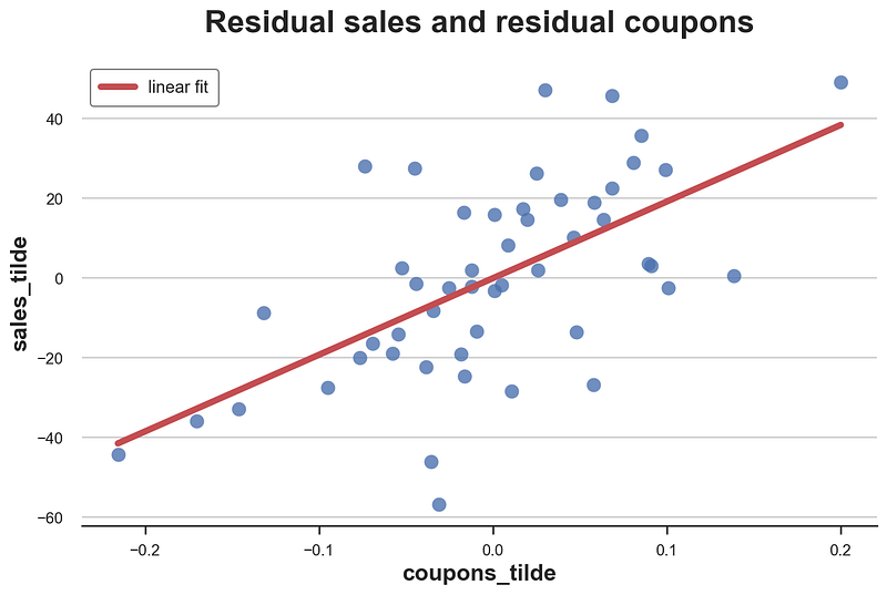

Now it’s evident from the graph that the conditional relationship (conditional on income) between sales and coupons is positive.

One problem with this approach is that the variables are hard to interpret: we now have negative values for both sales and coupons. Weird.

How did it happen? It happened because when we partialled-out the variables, we included the intercept in the regression, effectively de-meaning the variables (i.e. normalizing their values so that their mean is zero).

We can solve this problem by scaling both variables, adding their mean.

df['coupons_tilde_scaled'] = df['coupons_tilde'] + np.mean(df['coupons'])
df['sales_tilde_scaled'] = df['sales_tilde'] + np.mean(df['sales'])

Now the magnitudes of the two variables are interpretable again.

sns.regplot(x="coupons_tilde_scaled", y="sales_tilde_scaled", data=df, ci=False, line_kws={'color':'r', 'label':'linear fit'})
plt.legend()
plt.title(f"Residual sales scaled and residual coupons scaled");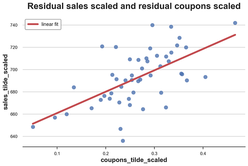

Is this a valid approach or did it alter our estimates? We can check it by running the regression with the scaled partialled-out variables.

smf.ols('sales_tilde_scaled ~ coupons_tilde_scaled', df).fit().summary().tables[1]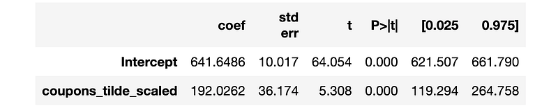

The coefficient is exactly the same as before!

Computational Speed

Another application of the Frisch-Waugh-Lovell theorem is to increase the computational speed of linear estimators. For example, it is used to compute efficient linear estimators in presence of high-dimensional fixed effects (day of the week in our example).

Some packages that exploit the Frisch-Waugh-Lovell theorem include

I also what to mention the fixest package in R, which is also exceptionally efficient in running regressions with high dimensional fixed effects, but uses a different procedure.

Inference and Machine Learning

Another important application of the FWL theorem sits at the intersection of machine learning and causal inference. I am referring to the work on post-double selection by Belloni, Chernozhukov, Hansen (2013) and the follow up work on “double machine learning” by Chernozhukov, Chetverikov, Demirer, Duflo, Hansen, Newey, Robins (2018).

I plan to cover both applications in future posts, but I wanted to start with the basics. Stay tuned!

References

[1] R. Frisch and F. V. Waugh, Partial Time Regressions as Compared with Individual Trends (1933), Econometrica.

[2] M. C. Lowell, Seasonal Adjustment of Economic Time Series and Multiple Regression Analysis (1963), Journal of the American Statistical Association.

Code

You can find the original Jupyter Notebook here.

Blog-Posts/fwl.ipynb at main · matteocourthoud/Blog-Posts

Code and notebooks for my blog posts. Contribute to matteocourthoud/Blog-Posts development by creating an account on…

github.com

Thank you for reading!

I really appreciate it! 🤗 If you liked the post and would like to see more, consider following me. I post once a week on topics related to causal inference and data analysis. I try to keep my posts simple but precise, always providing code, examples, and simulations.

Also, a small disclaimer: I write to learn so mistakes are the norm, even though I try my best. Please, when you spot them, let me know. I also appreciate suggestions on new topics!