The Fractal Dimension Index on Predicting Market Tops & Bottoms

Coding a Variation of the Fractal Dimension Index.

Markets are fractal in nature meaning they possess certain properties such as self-similarity that allows them to be modelled using tools from this field. Of course, this is easier said than done. In this article, we will try to develop the Fractal Dimension Index from the Hurst Exponent function in order to see how we can predict when market trends are about to break. We will first start by introducing and coding the Hurst Exponent before moving on to the Fractal Dimension Index.

I have just published a new book after the success of New Technical Indicators in Python. It features a more complete description and addition of complex trading strategies with a Github page dedicated to the continuously updated code. If you feel that this interests you, feel free to visit the below link, or if you prefer to buy the PDF version, you could contact me on Linkedin.

The Hurst Exponent

Financial assets alternate between momentum and mean-reversion as regimes and business cycles change. One way to know whether markets are mean-reverting or trending (thus momentum is prevailing) is to use the Hurst Exponent.

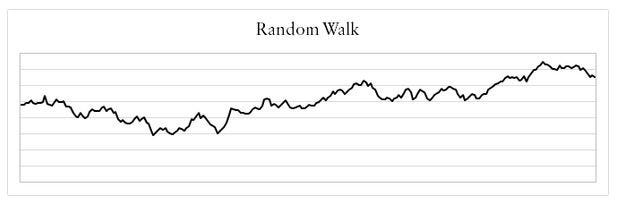
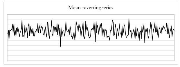
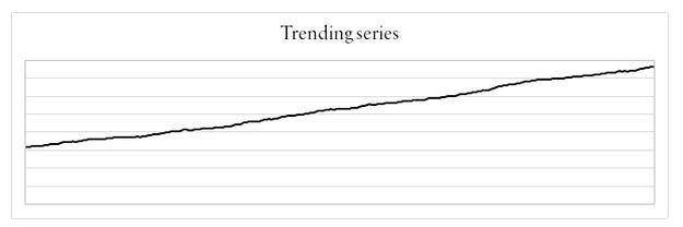
The three general types of financial data that can be observed are; trending, mean-reverting, and random walk.

• A Trending time series is one that increases or decreases over time. The main characteristic is positive autocorrelation.
• A Mean-reverting time series is one that fluctuates around its long-term equilibrium. The main characteristic is negative autocorrelation.
• A Random Walk time series is one that moves randomly over time. The main characteristic is zero autocorrelation.

The Random Walk theory is the foundation of quantitative finance and is one of the first things a practitioner should understand. Financial data are assumed to follow a random walk and that implies that price movements are random and cannot be forecasted using their past values. Our aim here is to understand which of the three types is the main characteristic of our analyzed data and that question can be answered through the Hurst exponent.

To briefly define this metric, it has been created by British hydrologist, Edwin Hurst during a study on the Nile river in Egypt. We can interpret it in the following three ways:

• Whenever H < 0.5, then we can say that our data is mean-reverting.
• Whenever H =0.5, then we can say that our data is random.
• Whenever H >0.5, then we can say that our data is trending in nature.

If we calculate the Hurst Exponent on real world data, for example the S&P500 index between 2007 and 2019, we find that it is around 0.43. Does this mean that the index is mean-reverting?

Not necessarily, the calculated value is from the 2007–2019 period and has a range of 30 values which may not capture the whole story. The true value should lie between 0.49 and 0.51 which is closer to a random walk with a pinch of determinism. We cannot negate the possibility that the S&P500 follows no specific pattern whatsoever and although we know that it does from time to time (mostly trending), we merely want to learn how to use the Hurst exponent for quick statistical tests granted we use quality data and optimal parameters such as taking relevant time periods. Another real example is the US M2 money supply. Naturally, it is always upwards sloping.

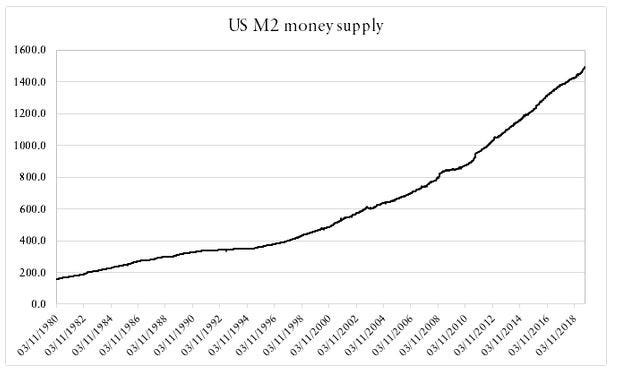
It is apparent that it is trending overtime, but what does the exponent say? According to the results shown, the Hurst exponent is around 0.744 which is an indication of a highly trending series. Mathematically speaking, the Hurst exponent revolves around the idea of using the variance of a log price series to determine the diffusion. What the function does is compare the diffusion of a time series to that of a geometric Brownian motion, in other words, if the data possesses autocorrelation then the below relationship will not hold and can be modified to include a value of 2H, which is actually the Hurst exponent:

If H = 0.5, then the equation would reduce to the below:

That is the rate of diffusion of a geometric Brownian motion. Tau (𝛕) denotes time and it is equal to the variance at a longer time horizon. The geometric Brownian motion dictates that the variance is equal to the time horizon when it is large enough. It becomes clear now why we say that when the Hurst exponent equals 0.5, we have a random time series.

To calculate a rolling measure of the Hurst Exponent, we need to first install the library:

pip install hurst

Next, we can create the function as below:

from hurst import compute_Hc

def hurst(Data, lookback, what, where):

for i in range(len(Data)):
        try:
            new = Data[i - lookback:i, what]
            
            Data[i, where] = compute_Hc(Data[i - lookback:i + 1, what])[0]
        except ValueError:
            pass
        
    return Data

# Using the Function
my_data = hurst(my_data, 100, 3, 4)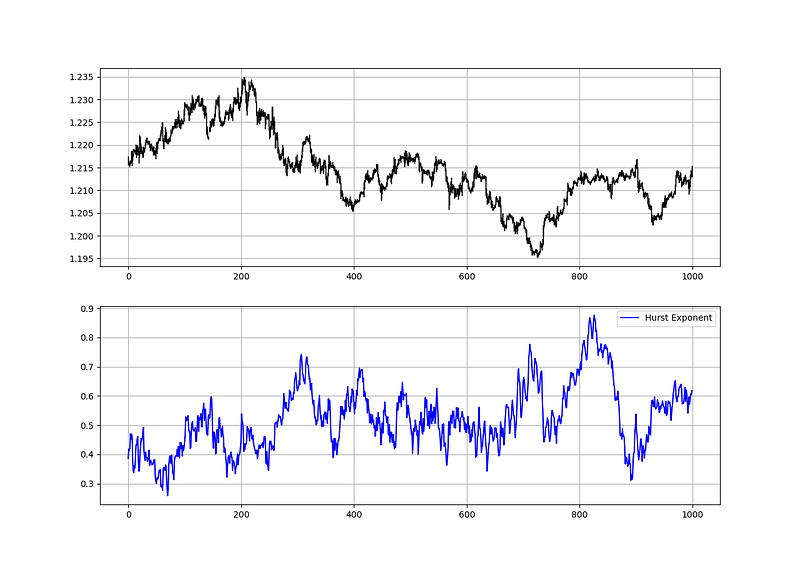

Whenever the market starts to trend, its Hurst Exponent starts to rise due to persistency until markets start to consolidate which is when the Hurst starts dropping. The idea of detecting tops in the Hurst to detect market turning points seems reasonable but in practice, it is not very useful as the Hurst does not really follow a clear stationary pattern. Yesterday’s 0.60 barrier is today’s meaningless level.

The Fractal Dimension Index

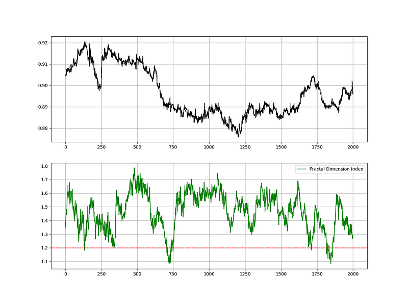
The index measures how irregular the time series is. When there is a strong trend going on, naturally, the market price is approaching a one-dimensional line and the Fractal Dimension Index approaches 1.0. When the market is choppy and moving sideways, the Fractal Dimension Index approaches 2.0.

The Fractal Dimension can be easily calculated from the Hurst Exponent using the following formula:

Therefore, the code can be adjusted to the following:

def fractal_dimension_index(Data, lookback, what, where):

for i in range(len(Data)):
        try:
            new = Data[i - lookback:i, what]
            
            Data[i, where] = compute_Hc(Data[i - lookback:i + 1, what])[0]
            Data[i, where] = 2 - Data[i, where]
            
        except ValueError:
            pass

    return Data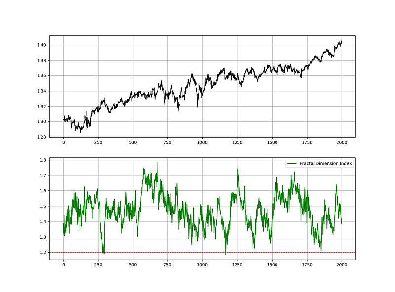

If you are also interested by more technical indicators and using Python to create strategies, then my best-selling book on Technical Indicators may interest you:

Using the Fractal Dimension Index

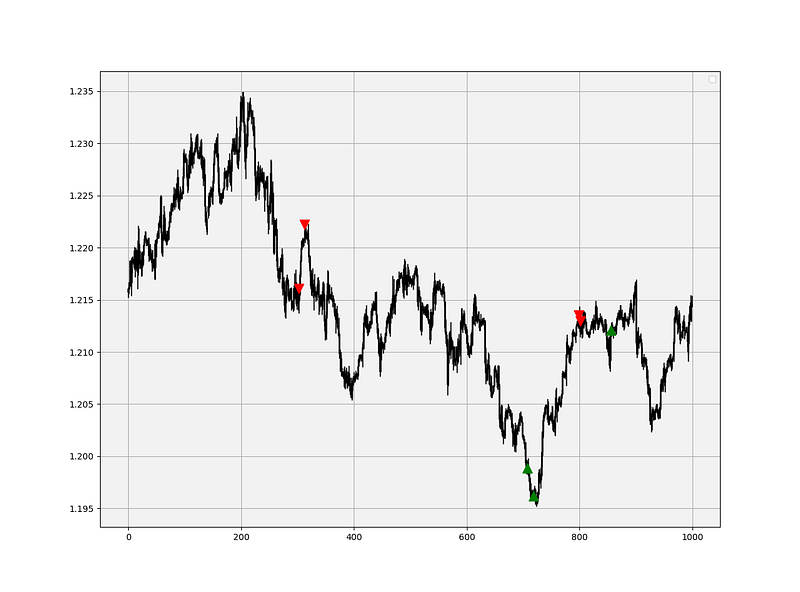
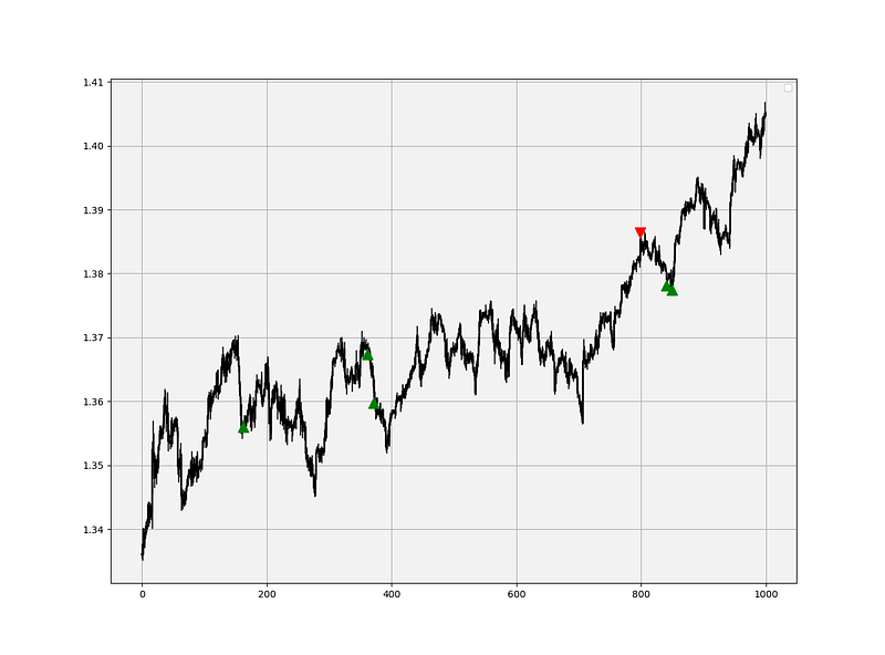
There is not really a clear trading strategy that can be formed around the Fractal Dimension Index. The best way is to check for extreme lows around 1.25/1.20 to see whether the current move will be broken or not. To put it in clear terms:

• Whenever the market is trending down and the Fractal Dimension Index reaches 1.25/1.20, we should be careful as we are probably entering a bottoming phase.
• Whenever the market is trending up and the Fractal Dimension Index reaches 1.25/1.20, we should be careful as we are probably entering a toppish phase.

Obviously, the index must be tweaked so that it delivers more signals. The main tweaks are the barriers and the addition of other technical indicators.

def signal(Data, fdi, trend, buy, sell):
    
  for i in range(len(Data)):
            
     if Data[i, fdi] < lower_barrier and Data[i, what] < Data[i - trend, what] and Data[i - 1, fdi] > lower_barrier:
            Data[i, buy] = 1
            
     if Data[i, fdi] < lower_barrier and Data[i, what] > Data[i - trend, what] and Data[i - 1, fdi] > lower_barrier:
            Data[i, sell] = -1

# The trend variable is to help the algorithm know whether the market has been trending up or down

A Throwback to the Hurst Exponent

How can we use the Hurst Exponent in trading, considering it does not have predictive properties?

Assume you have a performance period to assess after having used a strategy or model that comes from the family of trend-following systems and then you look at the Hurst of the performance period of the asset only to notice that is around 0.389 making it a mean-reverting time period. You can conclude that you cannot say the strategy used is bad, but that the market structure of the performance period was not convenient to the model and thus it is better to test it on a a trending market in order to fully know its profitability. What you know for sure is that the strategy you have is not adapted to all types of markets and that is already a useful information extracted from the Hurst.

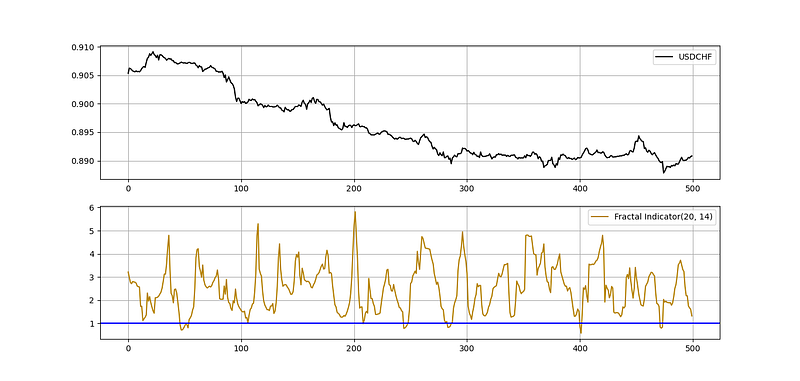
A Similar Tool: The Fractal Indicator

In a previous article, we have discussed the Fractal Indicator which is different from the one discussed above. British hydrologist Harold Edwin Hurst introduced a measure of variability of time series across the period of time analyzed. This measure is called the Rescaled Range Analysis which is the basis of our Fractal Indicator. Here is how to calculate Rescaled Range:

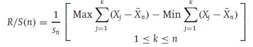
The Rescaled Range formula is very interesting as it takes into account the volatility (S), the mean (X-bar), and the range of the data to analyze its properties. What the above formula says is that, we have to calculate the range between the mini ranges of the maximum and minimum values and then divide them by the Standard Deviation, which in this case is the proxy for volatility.

As I am a perpetual fan of do-it-yourself and tweak-it-yourself, I have modified the formula to have the following sense which we will later see together in a step-by-step method:

Incorporating the highs and the lows could give us a clearer picture on volatility, which is why we will first calculate an exponential moving average on both the lows and highs for the previous X period and then calculate their respective standard deviation i.e. volatility. Next, we will calculate the first range where we will subtract the current high from the average high measured by the exponential moving average in the first step and then do the same thing with the low. After that, we will calculate a rolling maximum for the first range (the high minus its average) and a rolling minimum for the second range (the low minus its average). Then, we subtract the the high rolling maximum from the low rolling minimum before rescaling by dividing the result by the average between the two standard deviations calculated above for the highs and lows.

This is all done using the following function that requires an OHLC array with a few columns to spare:

def fractal_indicator(Data, high, low, ema_lookback, min_max_lookback, where):
    
    Data = ema(Data, 2, ema_lookback, high, where)
    Data = ema(Data, 2, ema_lookback, low, where + 1)
    
    Data = volatility(Data, ema_lookback, high, where + 2)
    Data = volatility(Data, ema_lookback, low, where + 3)
    
    Data[:, where + 4] = Data[:, high] - Data[:, where]
    Data[:, where + 5] = Data[:, low]  - Data[:, where + 1]for i in range(len(Data)):
        try:
            Data[i, where + 6] = max(Data[i - min_max_lookback + 1:i + 1, where + 4])
        
        except ValueError:
            pass              
        
    for i in range(len(Data)):
        try:
            Data[i, where + 7] = min(Data[i - min_max_lookback + 1:i + 1, where + 5])
        
        except ValueError:
            pass  
         
    Data[:, where + 8] =  (Data[:, where +  2] + Data[:, where +  3]) / 2
    Data[:, where + 9] = (Data[:, where + 6] - Data[:, where + 7]) / Data[:, where + 8]
    
    return Data

So, it becomes clear, the Fractal Indicator is simply a reformed version of the Rescaled Range formula created by Harold Hurst.

If you want to add columns to your array, you can use the below function:

def adder(Data, times):
    
    for i in range(1, times + 1):
    
        z = np.zeros((len(Data), 1), dtype = float)
        Data = np.append(Data, z, axis = 1)return Data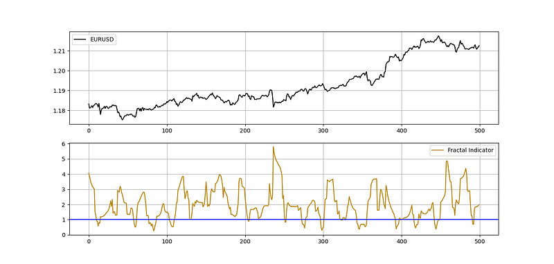

We have to understand how to use the Fractal Indicator. From charting, it is clear that we can find extreme values around the lower extremity which is 1.00 (or slightly lower depending on the parameters used below). We can call this, the Fractal Threshold.

Hence, a reasonable trading strategy can have the following conditions:

• Every time the Fractal Indicator reaches the 1.00 threshold while the market price has been trending downwards, we can expect that there will be a structural break in the market price, i.e. a short-term reversal to the upside. We should initiate a long position.
• Every time the Fractal Indicator reaches the 1.00 threshold while the market price has been trending upwards, we can expect that there will be a structural break in the market price, i.e. a short-term reversal to the downside. We should initiate a short position.

trend = 10
def signal(Data, what, closing, buy, sell):
    
    for i in range(len(Data)):
            
     if Data[i, what] < barrier and Data[i, closing] < Data[i - trend, closing]:
        Data[i, buy] = 1
            
     if Data[i, what] < barrier and Data[i, closing] > Data[i - trend, closing]:  
        Data[i, sell] = -1

# The trend variable is the algorithm's way to see whether the market price has been trending down or up. This is to known what position to initiate (long/short) as the Fractal Indicator only shows a uniform signal which is the event of reaching 1.00
# The Data variable refers to the OHLC array
# The what variable refers to the Fractal Indicator
# The closing variable refers to the closing price
# The buy variable refers to where we should place long orders
# The sell variable refers to where we should place short orders

It is worth noting that we can develop a miniature nomenclature to describe the Fractal Indicator. Notice how we have two variables, the lookback period on the exponential moving average and the lookback period on the normalization range period:

• The first variable is simply the moving average’s calculation period.
• The second variable is simply the range’s observation period.

Hence, a Fractal Indicator with an exponential moving average period of 20 and a normalization lookback period of 14 can be written as FI(20, 14).

We need the Exponential Moving Average function for the above indicator to work. It can be found here:

def ma(Data, lookback, what, where):
    
    for i in range(len(Data)):
      try:
        Data[i, where] = (Data[i - lookback + 1:i + 1, what].mean())
        
            except IndexError:
                pass
    return Data

def ema(Data, alpha, lookback, what, where):
    
    # alpha is the smoothing factor
    # window is the lookback period
    # what is the column that needs to have its average calculated
    # where is where to put the exponential moving average
    
    alpha = alpha / (lookback + 1.0)
    beta  = 1 - alpha
    
    # First value is a simple SMA
    Data = ma(Data, lookback, what, where)
    
    # Calculating first EMA
    Data[lookback + 1, where] = (Data[lookback + 1, what] * alpha) + (Data[lookback, where] * beta)

    # Calculating the rest of EMA
    for i in range(lookback + 2, len(Data)):
            try:
                Data[i, where] = (Data[i, what] * alpha) + (Data[i - 1, where] * beta)
        
            except IndexError:
                pass
    return Data

Conclusion

Why was this article written? It is certainly not a spoon-feeding method or the way to a profitable strategy. If you follow my articles, you will notice that I place more emphasize on how to do it instead of here it is and that I also provide functions not full replicable code. In the financial industry, you should combine the pieces yourself from other exogenous information and data, only then, will you master the art of research and trading.

I always advise you to do the proper back-tests and understand any risks relating to trading.