The Fisher Aggregate Index. Detecting Market Tops & Bottoms With Accuracy.

Squeezing out the best of the Fisher Transformation.

The incredible Fisher Transformation can also be “transformed” in order to enhance its signals. In this article, we will discuss the Fisher Transformation and then from it, create the Fisher Aggregate Index, a contrarian technical indicator used to detect market inflections.

I have just published a new book after the success of New Technical Indicators in Python. It features a more complete description and addition of complex trading strategies with a Github page dedicated to the continuously updated code. If you feel that this interests you, feel free to visit the below link, or if you prefer to buy the PDF version, you could contact me on Linkedin.

The Fisher Transformation

One of the pillars of descriptive statistics is the normal distribution curve. It describes how random variables are distributed and centered around a central value. It often resembles a bell. Some data in the world are said to be normally distributed. This means that their distribution is symmetrical with 50% of the data lying to the left of the mean and 50% of the data lying to the right of the mean. Its mean, median, and mode are also equal as seen in the below curve.

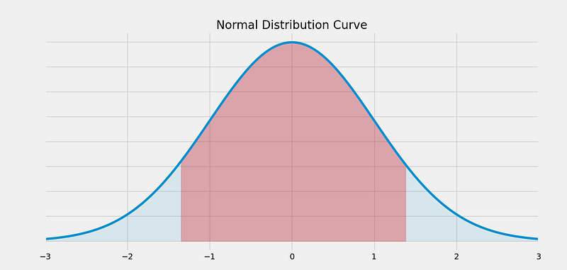
The above curve shows the number of values within a number of standard deviations. For example, the area shaded in red represents around 1.33x of standard deviations away from the mean of zero. We know that if data is normally distributed then:

• About 68% of the data falls within 1 standard deviation of the mean.
• About 95% of the data falls within 2 standard deviations of the mean.
• About 99% of the data falls within 3 standard deviations of the mean.

Presumably, this can be used to approximate the way to use financial returns data, but studies show that financial data is not normally distributed. For the moment, we can assume it is so that we can use such indicators. The flaw of the method does not hinder much its usefulness.

Let us now see how to create the Modified Fisher Transformation which is basically like the original one but with some minor changes to enhance the results and make them easier to obtain.

Created John F. Ehlers, the indicator seeks to transform the price into a normal Gaussian (normal) distribution. This is very helpful in detecting reversals which is the main point of the article. The steps to create the Modified Fisher Transformation are somewhat similar to the original Fisher Transformation. Here is how we do it:

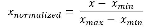
• Select a lookback period and calculate a normalized version of the OHLC data using the original Stochastic formula as seen in the formula below:

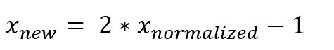
• Trap the values from the first step between -1 and +1 using the following normalization formula:

• Create a condition that eliminates the -1.00’s and +1.00’s and transforms them into -0.999’s and +0.999’s so that we do not get infinite values. This also serves to make the indicator bounded between two levels we will see later.
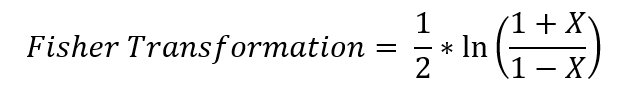
• Apply the following formula to the results from the last step:

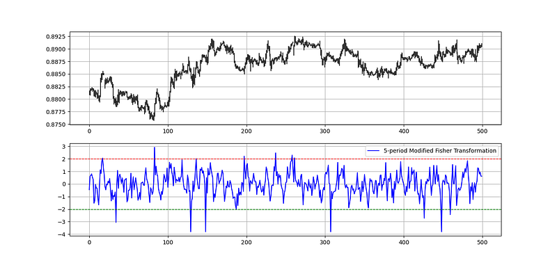
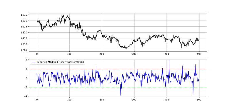
Now that we have the Modified Fisher Transformation Indicator, we can proceed by coding it in Python before starting the back-tests. The below plot shows a 5-period Modified Fisher Transformation with subjective boundaries at -2.00 and +2.00.

def stochastic(Data, lookback, what, where):
        
    for i in range(len(Data)):
        
        try:
            Data[i, where] = (Data[i, what] - min(Data[i - lookback + 1:i + 1, 2])) / (max(Data[i - lookback + 1:i + 1, 1]) - min(Data[i - lookback + 1:i + 1, 2]))
        
        except ValueError:
            pass
    Data[:, where] = Data[:, where] * 100  

    return Data

def modified_fisher_transform(Data, lookback, what, where):
    
   Data = stochastic(Data, lookback, what, where)
   Data[:, where] = Data[:, where] / 100
   Data[:, where] = (2 * Data[:, where]) - 1
   
   for i in range(len(Data)):
       if Data[i, where] == 1:
           Data[i, where] = 0.999
       if Data[i, where] == -1:
           Data[i, where] = -0.999
           
   for i in range(len(Data)):
       
      Data[i, where + 1] = 0.5 * (np.log((1 + Data[i, where]) / (1 - Data[i, where])))  
   
   return Data

# Using the Transformation on an OHLC array with a few extra columns
my_ohlc_data = modified_fisher_transform(my_ohlc_data, 5, 3, 4)

Naturally with the correction I have added, the maximum values will be 3.80 and the minimum values will be -3.80. Therefore, we can say that the indicator is now bounded even though the original version was not shown to be bounded.

Let us first define some primal functions that make the data manipulation easier:

# The function to add a certain number of columns
def adder(Data, times):
    
    for i in range(1, times + 1):
    
        z = np.zeros((len(Data), 1), dtype = float)
        Data = np.append(Data, z, axis = 1)                   

    return Data

# The function to deleter a certain number of columns
def deleter(Data, index, times):
    
    for i in range(1, times + 1):
    
        Data = np.delete(Data, index, axis = 1)               

    return Data

# The function to delete a certain number of rows from the beginning
def jump(Data, jump):
    
    Data = Data[jump:, ]
    
    return Data

The Fisher Aggregate Index

The Fisher Aggregate Index seeks to gather as much extremes as possible from a range of lookback periods. This means that we will calculate the Modified Fisher Transformation using a set of different lookback periods and then average them all out.

We can try out a range between a 3-period Fisher and a 29-period Fisher. This can be coded as the below:

where = 4
for i in range(3, 30):
    
    my_data = fisher_transform(my_data, i, 3, where)
    where = where + 1

my_data= adder(my_data, 1)

for i in range(len(my_data)):

    my_data[i, -1] = np.sum(my_data[i, 4:4+ 30 - 3])
    my_data[i, -1] = my_data[i, - 1] / (30 - 3)

my_data = deleter(my_data, 4, 27)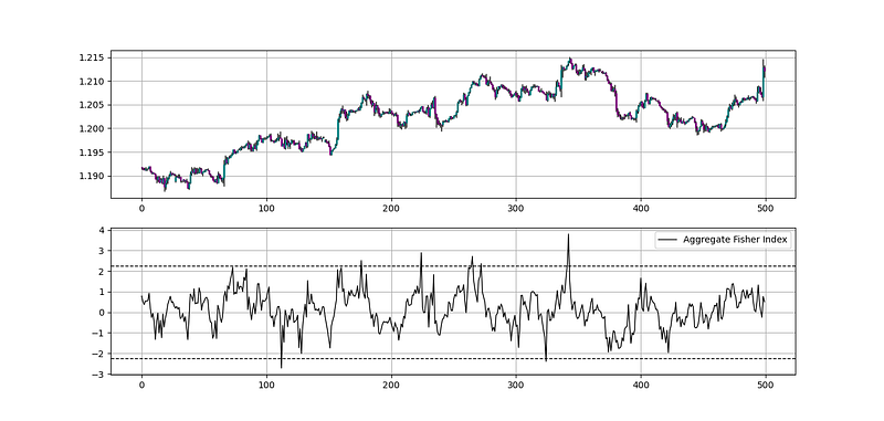  

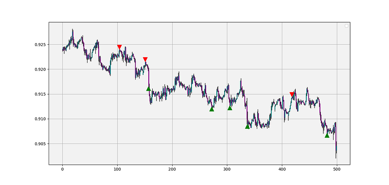
The below shows the signals generated using the index. The conditions are below.

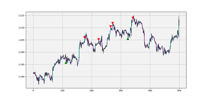
If we want to follow the barriers technique where we buy around support and go short around resistance, then we can try out the following conditions:

• Go long (Buy) whenever the Fisher Aggregate Index reaches the lower barrier with the two previous readings higher than the lower barrier. Hold this position until getting a new signal or getting stopped out by the risk management system.
• Go short (Sell) whenever the Fisher Aggregate Index reaches the upper barrier with the two previous readings lower than the upper barrier. Hold this position until getting a new signal or getting stopped out by the risk management system.

upper_barrier = 2.24
lower_barrier = -2.24

def signal(Data, what, buy, sell):
    
    for i in range(len(Data)):
            
        if Data[i, what] < lower_barrier and Data[i - 1, what] > lower_barrier and Data[i - 2, what] > lower_barrier :
            Data[i, buy] = 1
            
        if Data[i, what] > upper_barrier and Data[i - 1, what] < upper_barrier and Data[i - 2, what] < upper_barrier :
            Data[i, sell] = -1    
            
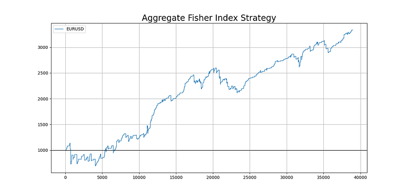
    return Data

The choice of the barriers were to make a zone around the 2.00 graphical level. 2.24 equals the sum of the golden ratio and its reciprocal. The below is a back-testing result on the EURUSD using hourly data since 2015 with a spread of 0.5 and a theoretical risk-reward ratio of 0.20.

If you are also interested by more technical indicators and using Python to create strategies, then my best-selling book on Technical Indicators may interest you:

Conclusion

Remember to always do your back-tests. Even though I supply the indicator’s function (as opposed to just brag about it and say it is the holy grail and its function is a secret), you should always believe that other people are wrong. My indicators and style of trading work for me but maybe not for everybody. I rely on this rule:

The market price cannot be predicted or is very hard to be predicted more than 50% of the time. But market reactions can be predicted.

What the above quote means is that we can form a small zone around an area and say with some degree of confidence that the market price will show a reaction around that area. But we cannot really say that it will go down 4% from there, then test it again, and breakout on the third attempt to go to $103.85. The error term becomes exponentially higher because we are predicting over predictions.

To sum up, are the strategies I provide realistic? Yes, but only by optimizing the environment (robust algorithm, low costs, honest broker, proper risk management, and order management). Are the strategies and indicators provided only for the sole use of trading? No, it is to stimulate brainstorming and getting more trading ideas as we are all sick of hearing about an oversold RSI as a reason to go short or resistance being surpassed as a reason to go long. I am trying to introduce a new field called Objective Technical Analysis where we use hard data to judge our techniques rather than rely on outdated classical methods.