
The Financial Market Crash of 1929: Explained Computationally

The Wall Street Crash of 1929 occurred in late October 1929 at the New York Stock Exchange (NYSE).
In the span of a week, stock market share values collapsed. The events known as Black Thursday and Black Tuesday triggered a decade of severe economic decline both in the U.S. and around the world, which came to be known as the Great Depression.
The causes can be linked to the laissez-faire approaches to market speculation, i.e. loose regulation, and the situations of panic-selling created the circumstances for the greatest economic collapse in the modern world economy.
The Crash Explained
Increase in Urbanization — Decrease in Agricultural Output
The end of World War I in 1918 brought about a major boost in the economy in the United States in terms of expansion of urbanization, industrialization and financial investment in consumer goods industries.
This urbanization, however, came at the cost of the rural agricultural communities that saw major shortages in employable, skilled workers. As a result, agricultural output and farming communities suffered substantial losses during this period.
The 1920s are perhaps best characterized by the extravagance of urban populations who enjoyed lavish lifestyles and were willing to invest in highly speculative offerings on the NYSE.
The laissez-faire financial policy, marked by minimal regulation and control, of the Hoover administration, despite the declining gross domestic product and the ongoing decline in agriculture and rural economics, remained confident in its non-interventionist approach. This created an economic bubble whereby confidence was not based on rational methods of understanding stock fluctuations, but rather on the personal confidence that investors had in the pathway of the stock exchange.
The Lead Up
In the 1920’s there was an overarching belief that the American economy would continue to grow, however, by the end of the decade, steel production, construction and agricultural output were slowing down, while easy credit meant that the housing, consumer goods and automobile markets were expanding at an unsustainable rate.
On March 29th 1929 when the Federal Reserve sent a warning about excessive speculation in equities, something that sent a few investors wanting to protect, and therefore, sell their investments, causing a dip in the NYSE. The dip recovered soon after, but the underlying economic problems remained.
In September 1929, a high-profile British investor was jailed for fraud and stock manipulation on the London Stock Exchange. This sent the stock exchange into turmoil and caused a serious loss of confidence in foreign investment from the NYSE.
The Crash
On October 24th 1929 the market lost 11% on a single day of trading with very heavy trading volume.
On October 28th, many investors decided to leave the market as confidence began to slip in the declining Dow Jones Industrial Index and the overall health of the NYSE. The stock exchange slipped by a further 13% and newspapers reported the losses across the country, furthering the decline in financial confidence.
On October 29th, panic-selling hit its all-time high and the market collapsed as investors refused to buy stocks and dumped their remaining investments wherever they could.
Charting the Build-Up and Crash
Volumes, Regimes and Liquidity
Markets are complex and dynamic systems made up of many agents who not only respond to external information, but to the market itself.
These agents learn over time and develop complex behaviour through their interactions. As these markets evolve, characteristics can change requiring new strategies in order to keep up with market trends.
Markets are dynamic and can me made up of a number of states. Markets can often respond and behave dramatically different during times of crisis, that they do in either Bull or Bear Markets.
While price is a significant concern for investor performance, so too is liquidity.
As market information changes, we can often observe the market forces of supply and demand push and pull, as investors rapidly move to buy and sell-off holdings based on their own investment strategies and fast-changing market information.
While liquidity, as a concept, is something difficult to directly quantify, for many investors volume can provide an interesting insight over time into changes to market information, demand and supply and liquidity.
When volumes are lower than normal that can often signal little changes in market information when volumes are high, information can be changing dramatically, forcing investors to alter their portfolios and investment strategies.
From the diagram below, we plot Volume for the NYSE from 1888 to 1979 over time.
Downloading and Loading the Data
# Import Libraries
import os
import requests
import pandas as pd
import numpy as npimport holoviews as hv
import hvplot.pandas# Import Plotting Backend
hv.extension('bokeh')date_ranges = [[1970, 1979, 'dat'],
[1960, 1969, 'dat'],
[1950, 1959, 'dat'],
[1940, 1949, 'dat'],
[1930, 1939, 'dat'],
[1920, 1929, 'prn'],
[1900, 1919, 'dat'],
[1888, 1899, 'dat']][::-1]We download the data for each decade — for example 1920–1929 — and save this data in the folder Data that we create in the same location we have our notebook.
# Download Datadef get_decade(start = 1920, end = 1929, extension='prn'):
"Specify the starting year of the decade eg. 1900, 2010, 2009"
try:
link = requests.get(f'https://www.nyse.com/publicdocs/nyse/data/Daily_Share_Volume_{start}-{end}.{extension}')
file = os.path.join(".","Data",f"Daily_Share_Volume_{start}-{end}.{extension}")
if link.status_code == 404:
raise
else:
with open(file, 'w') as temp_file:
temp_file.write(str(link.content.decode("utf-8")))print(f"Successfully downloaded {start}-{end}")except:
print("There was an issue with the download. \n\
You may need a different date range or file extension. \n\
Check out https://www.nyse.com/data/transactions-statistics-data-library")download_history = [get_decade(decade[0], decade[1], decade[2]) for decade in date_ranges]We can then load the data:
# Read and format the data
def load_data(start = 1920, end = 1929, extension='prn'):
    path = os.path.join(".","Data",f"Daily_Share_Volume_{start}-{end}.{extension}")

    if extension=='prn':
        data = pd.read_csv(path , sep='   ', parse_dates=['Date'], engine='python').iloc[2:,0:2]
        data.loc[:,"  Stock U.S Gov't"] = pd.to_numeric(data.loc[:,"  Stock U.S Gov't"], errors='coerce')
        data.Date = pd.to_datetime(data.Date, format='%Y%m%d', errors='coerce')
        data.columns = ['Date','Volume']
        return data
    else:
        data = pd.read_csv(path)
        data.iloc[:,0] = data.iloc[:,0].apply(lambda x: str(x).strip(' '))
        data = data.iloc[:,0].str.split(' ', 1, expand=True)
        data.columns = ['Date','Volume']
        data.loc[:,"Volume"] = pd.to_numeric(data.loc[:,"Volume"], errors='coerce')
        data.Date = pd.to_datetime(data.Date, format='%Y%m%d', errors='coerce')
        return data
data = pd.concat([load_data(decade[0], decade[1], decade[2]) for decade in date_ranges], axis=0)Plotting the Data
It is clear that volumes have increased dramatically over time, with increasing volatility and kurtosis. While we may speculate around the effect of increased market size, computerized trading and even high-frequency trading, it is interesting to note the dramatic changes markets experience during crisis situations.
Plotting the Volume
# Create plotting object
plot_data = hv.Dataset(data, kdims=['Date'], vdims=['Volume'])
# Create scatter plotblack_tuesday = pd.to_datetime('1929-10-29')vline = hv.VLine(black_tuesday).options(color='#FF7E47')m = hv.Scatter(plot_data).options(width=700, height=400).redim('NYSE Share Trading Volume').hist() * vline * \
hv.Text(black_tuesday + pd.DateOffset(months=10), 4e7, "Black Tuesday", halign='left').options(color='#FF7E47')
m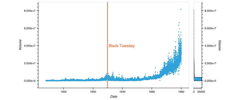
We see over a period of time, both before and after Black Tuesday, volumes become increasingly volatile as traders seek to price in the drama of new information. The feature of leverage, new to this market crash, forced many traders to alter their positions in the market in hope of settling margin accounts and hold onto trades.
Zooming in to the Relevant Decade
# Create plotting object
plot_data_zoom = hv.Dataset(data.loc[((data.Date >= pd.to_datetime("1920-01-01"))&(data.Date <= pd.to_datetime("1940-01-01"))),:], kdims=['Date'], vdims=['Volume'])
# Create scatter plotblack_tuesday = pd.to_datetime('1929-10-29')vline = hv.VLine(black_tuesday).options(color='#FF7E47')m = hv.Scatter(plot_data_zoom).options(width=700, height=400).redim('NYSE Share Trading Volume').hist() * vline * \
hv.Text(black_tuesday + pd.DateOffset(months=10), 4e7, "Black Tuesday", halign='left').options(color='#FF7E47')
m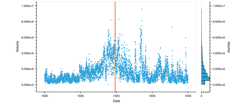
Autocorrelation Analysis
%%opts Bars [width=400 height=300]
from statsmodels.tsa.stattools import acf, pacf
def auto_correlations(start_year, window_years):
start_year = pd.to_datetime(f'{start_year}-01-01')
window_years = pd.DateOffset(years=window_years)
data_window = data
data_window = data_window.loc[((data_window.Date>=start_year)
&(data_window.Date<=(start_year+window_years))),:]
return hv.Bars(acf(data_window.Volume.interpolate().dropna()))\
.redim(y='Autocorrelation', x='Lags') +\
hv.Bars(pacf(data_window.Volume.interpolate().dropna()))\
.redim(y='Patial Autocorrelation', x='Lags').options(color='#FF7E47')hv.DynamicMap(auto_correlations,kdims=['start_year', 'window_years']
).redim.range(start_year=(data.Date.min().year,data.Date.max().year), window_years=(1,25))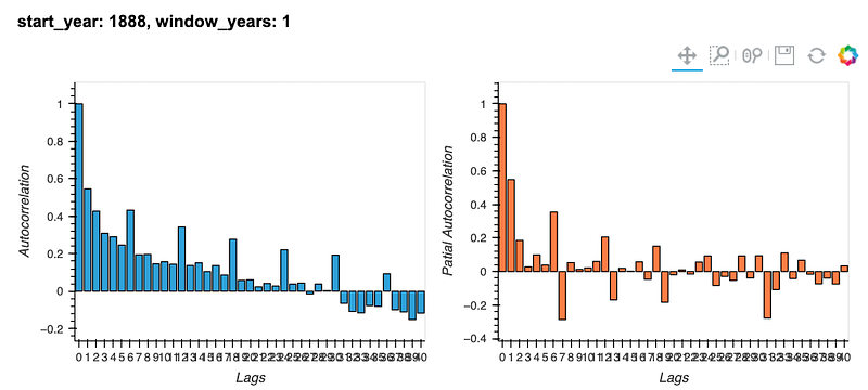
We can model this data in a rudimentary fashion, looking at the partial auto-correlation and auto-correlation present in this data.
These properties can vary dramatically over time and provide insight into the variance, efficiency and responsiveness of the market.
Many markets in developing economies can feature low levels of liquidity, even for large stocks. With large public investment companies and retail investors, changes in investment strategy can subsume liquidity in the market, as large volumes of trades look to be executed.
In these markets, these trades force the price to increase over many days and may result in increases in one or two-day auto-correlation depending on the characteristics of market liquidity.
These characteristics of momentum can also form part of investor strategy, or describe some element of market microstructure, but interesting to note from these plots above is how in recent years auto-correlation of volumes has seen radical changes to historical norms.
Generally, in these plots above, we can observe some inkling of these properties in the Partial Auto-correlation Plot, which displays a regular 2-day correlation indicative of characteristics of momentum and liquidity.
Code References and Explanation
World Quant University — Cases in Risk Management 2019
Modeling the Depression and Margin
Modeling market characteristics can be a hard task for historical market events. The lack of data can limit the methods and insights founds, and noise and exogenous factors can often obfuscate key and important insights.
However, simulation is a crucial technique in the understanding of complex systems which can help us gain insight into the effects which different investor heuristics have on markets.
Simulation can come in a number of different forms, Monte Carlo Simulation is one used extensively in computing VaR and Expected Shortfall for investor portfolios and can be used in pricing a number of complex derivatives and share options schemes.
from functools import reduce
import operator
import os
import requestsimport pandas as pd
import numpy as npimport holoviews as hv
import hvplot.pandasnp.random.seed(42)hv.extension('bokeh')Modeling Random Walks
The concept of random walks in prevalent in financial theory. They are used as assumptions in the efficient market hypothesis, capital asset pricing model and Black-Scholes option pricing formula, to name a few. Despite its use, most markets exhibit very different distributional properties — often displaying fatter tails, with far larger jumps and swings.
Below, we can graph these random walks, adjusting their parameters, 𝜇 and 𝜎 to allow for trend or different levels of volatility.
It is important to understand that not all random walks are alike and as you increase the number of walks you sample, you will see clearly how different they can be.
def plot(mu, sigma, samples):
    return pd.Series(np.random.normal(mu,sigma, 1000)).cumsum(
    ).hvplot(title='Random Walks', label=f'{samples}')
def prod(mu, sigma, samples):
return reduce(operator.mul,
list(map(lambda x: plot(mu,sigma, x),
range(1,samples+1))))hv.DynamicMap(prod,kdims=['mu', 'sigma', 'samples']).redim.range(mu=(0,5), sigma=(1,10), samples=(2,10)).options(width=900, height=400)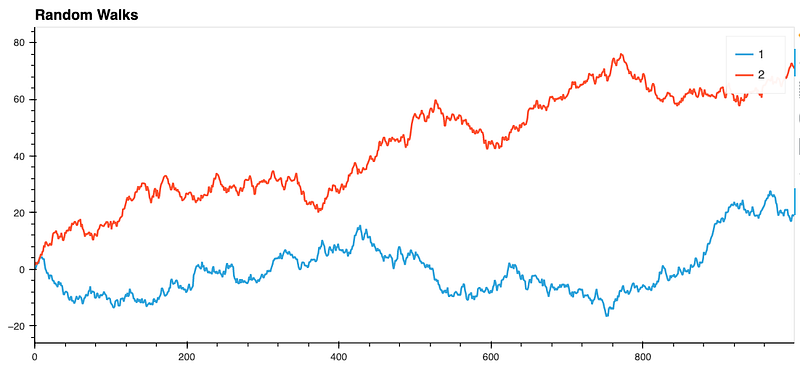
Capturing Market Dynamics
We will create a function that produces a random walk with 𝜇 and 𝜎 as some function of momentum (affecting 𝜇) and the number of market participants (affecting 𝜇 and 𝜎) who get introduced and removed from the market based on the activity of their Margin Accounts.
We will initialise a set of 100 with margin accounts, with varying levels of risk. In order for margin calls to affect the market, we will say that if their accounts dip below the margin level, they are ordered to sell, this will increase supply and decreases pries in the market though the Law of Supply and Demand and the market 𝜇 will be affected with some decay over the next n times steps.
As margin accounts are called, the characteristics of our random walk will change, and these traders will remain outside the simulation until randomly reintroduced.
Obviously if many default at the same time, it will take a long time for them to be reintroduced to the market and for prices to stabilise, if few default they should be reintroduced quickly as new participants arrive in the market to take advantage of mispricing.
As margin calls affect the 𝜇 of our random walk, we should see dramatic pull-downs as this affects other traders in the market.
After initialising the Accounts class, the price function starts by calculating the % of Margin Accounts that have been called at a given day and the 5-day Momentum in the market (𝑃{𝑡}−P{t−5}). Using these values and our simulation parameters, these values are used to compute 𝜇 and 𝜎 for our next market return.
The number of accounts called is then updated, given we now know the returns of the market on this given day. After this updating, we then randomly reinitialise called accounts, to signify new participants entering or re-entering the market.
class Accounts:
def __init__(self, account_mu=20, account_sigma=5, account_numbers=100, mu=0, sigma=0.05, margin_mu=0.1, momentum_mu=0.025, margin_sigma=0.001):
# We initialize paramters for our simulations
self.account_mu=account_mu
self.account_sigma = account_sigma
self.account_numbers = account_numbers
self.margin_mu=margin_mu
self.momentum_mu=momentum_mu
self.margin_sigma=margin_sigma
self.accounts= np.maximum(np.random.normal(loc=self.account_mu, scale=self.account_sigma, size = self.account_numbers),0)
self.call=self.accounts*np.random.uniform(0.5,0.7,self.account_numbers)
self.mu=mu
self.sigma=sigma
self.called_accounts_factor = 0
self.momentum = 0
self.history = [0,0,0,0,0]
return None
def price(self):
# Calculate factors
self.called_accounts_factor =((self.accounts <= self.call).sum())/self.account_numbers
self.momentum = (self.history[4] - self.history.pop(0))
# Update paramteres
self.mu = self.mu - self.margin_mu*self.called_accounts_factor + self.momentum_mu*self.momentum
self.sigma = self.sigma + self.margin_sigma*self.called_accounts_factor
# Update accounts
self.history.append(np.random.normal(loc=self.mu, scale=self.sigma))
self.accounts = self.accounts*(1+self.history[4]*np.random.uniform(low=0.5,high=1.5,size=self.account_numbers))
# Reset called accounts
reset = (np.random.rand(self.account_numbers)>=0.3) * (self.accounts <= self.call)
self.accounts[reset] = np.random.normal(self.account_mu, self.account_sigma)
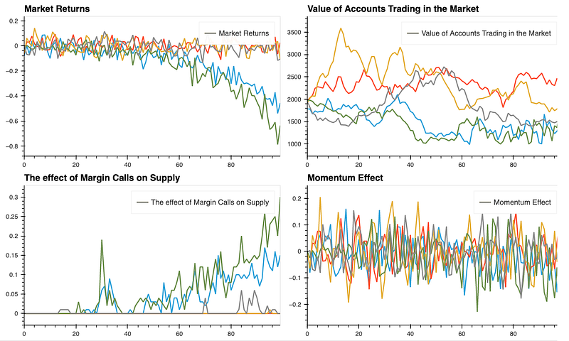
self.call[reset] = self.accounts[reset]*np.random.uniform(0.2,0.5,np.sum(reset))return [self.history[4], self.accounts.sum(), self.called_accounts_factor, self.momentum]We will run this simulation over 100 days, and produce five different runs of this simulation to get an idea of the possible outcomes this simulation produces.
We will keep track of the Market Returns, the Average Value of our Margin Accounts, the Number of Accounts called at a given point in time, and the effect they will have on the distribution of returns, as well as the momentum effect we will be used to affect the distribution of returns as well.
def simulation_plots(days=10000, runs=5):
    run = []

    for _ in range(runs):
        a = Accounts()
        prices = pd.DataFrame([a.price() for day in range(days)],
                              columns=['Market Returns', 'Value of Accounts Trading in the Market', 'The effect of Margin Calls on Supply', 'Momentum Effect'])
        run.append(prices)

    plot = reduce(operator.mul,[i.iloc[:,0].hvplot() for i in run]) +\
            reduce(operator.mul,[i.iloc[:,1].hvplot() for i in run]) +\
            reduce(operator.mul,[i.iloc[:,2].hvplot() for i in run]) +\
            reduce(operator.mul,[i.iloc[:,3].hvplot() for i in run])


    return plot.cols(2)
In these graphs, each line represents a run of the simulation over the intended number of days. These are presented in different colours to aid in readability. The four panes of the plot represent: Market Returns, Value of Accounts Trading in the Market, The effect of Margin Calls on Supply and a Momentum Effect.
Comparison with Normal Distribution
From these graphs, we can see how volatile returns appear.
Unlike white noise, these feature strong violent trends.
Margin Calls take place dramatically for almost all participants in the market like a set of dominoes and momentum tends to carry these effects, as traders panic.
def simulation_prices(days=100, runs=1000, axis=0):
    run = []

    for _ in range(runs):
        a = Accounts()
        prices = pd.DataFrame([a.price()[0] for day in range(days)],
                              columns=['return'])
        run.append(prices)


    output = pd.concat(run, axis=axis)
    output.columns = [f'Run {i+1}' for i in range(output.shape[1])]

    return output
simulations = simulation_prices()%%opts Overlay [show_title=True] Distribution [height=500, width=1000]
hv.Distribution(np.random.normal(simulations.mean(),simulations.std(),100000), label='Normal') * hv.Distribution(simulations.iloc[:,0], label='Simulation').options(fill_alpha=0.0)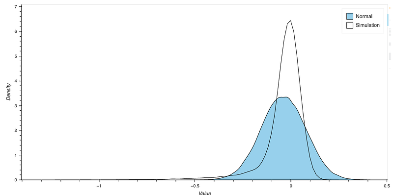
Looking at the graphs above, when we compare this simulation against the standard Normal Distribution and a Normal Distribution with equal mean and variance properties.
We see noticeably different characteristics. Our models appear both skew and spread out, with far higher probabilities for events well outside the Standard Normal Distribution; we used as our original function. While it still appears approximately normal, if we compare it to a normal distribution with similar mean and variance characteristics, we do appear to have far higher levels of kurtosis- indicated by the higher mode of the distribution and the longer left tail.
This longer left tail of this distribution seems to indicate additional skewness to the distribution, which may form an interesting characteristic for investors to consider.
Code References and Explanation
World Quant University — Cases in Risk Management 2019

This Article is published on The Quant Journey, an initiative started to take the readers along side this journey towards learning about quantitative finance topics.
Check out our Instagram Page: The Quant Journey
