GNNs Explained Series

The Expressive Power of GNNs — Introduction and Foundations

Connecting the dots for a theoretical analysis of Graph Neural Network models

This series aims to provide a comprehensive understanding of how GNNs capture the relational information of network structures.

Introduction

Graphs represent universal models to describe interacting elements, and Graph Neural Networks (GNNs) have become an essential toolkit for applying learning algorithms to graph-structured data.

The most common framework of GNNs is based on the Message Passing Neural Network (MPNN). In this framework, the neighbor features are passed to the target node as messages through the edges. Then, the target node representation is updated with the aggregated representation of its neighbors.

Based on this principle, the new representation of the node encodes information related to the local structure. This message-passing procedure is illustrated in Figure 1.

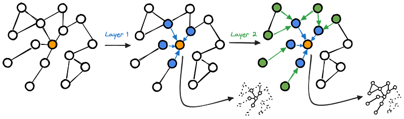
Figure 1 — Aggregation of neighbor features into the orange node in a 2-layer MPNN

This Figure shows how the representation of the orange node is updated, aggregating its neighbors' features. More specifically, by stacking a single MPNN layer, the orange node is updated with the representation of the blue nodes. Adding one more layer, the resulting representation of the orange node incorporates the features of blue and green nodes.

For the sake of simplicity, we are considering only the aggregation performed on the orange node. However, this computation is executed in parallel for all the nodes in the graph, including the blue and the green nodes, whose representation is updated with their neighbor (including the orange one!) features.

The main difference between diverse MPNN models lies in the type of feature aggregation executed to update the node representation. The neighbor features can be aggregated using a sum or an average operation, as in the case of Graph Convolutional Networks (GCNs) and GraphSage. In other cases, such as Graph Attention Networks (GATs), we can add a further step in which the contribution of each neighbor node is weighted according to its importance.

Further details on such updating/aggregation operations are available in the following articles, which include Python code examples:

Understanding the Building Blocks of Graph Neural Networks (Intro)

An intuition (with running code) on the framework to analyze and learn graph data with neural architectures

towardsdatascience.com

Graph Attention Networks Under the Hood

A Step-by-step Guide From Math to NumPy

towardsdatascience.com

Article Series Details

A GNN model requires the ability to encode distinct representations for graphs characterized by diverse structures. Similarly, such a model should be able to encode the same representation for graphs with the same relational structure. This series aims to provide all the details for consistently measuring this ability by building intuitions and showing running code.

The series is articulated as follows:

This introductory article sets the foundations. It describes how to represent graphs and discusses the critical idea of graph isomorphism, which is essential to clarifying the concept of distinct or equivalent relational structures.
The second article showcases the concepts of equivariance and invariance, building intuition on image data and then applying these concepts to graphs. Comprehending these notions will allow us to understand how GNN models work from this perspective.
The third article introduces the Weisfeiler-Leman (WL) algorithm, a color refinement method to test graph isomorphism, and clarifies how this algorithm is connected to the expressive power of GNNs.
The fourth article shows experiments to compare the expressivity of different GNN models on a graph classification task by combining all the ingredients built in the previous three articles.

Let’s start our journey with the key foundations. First, we will focus on graph representation using vectors, matrices, and tensors. Second, we will build intuition and clarify the idea of graph isomorphism, from sketched diagrams to a formal definition. Finally, we will connect the two previous points, explaining the concept of graph isomorphism in terms of adjacency and permutation matrices.

Graph Representation

We can introduce graphs as mathematical objects that allow us to model relational data. Traditionally, we can define a graph with the following notation: G = (V, E), where V represents the set of vertices (or nodes), while E represents the set of edges.

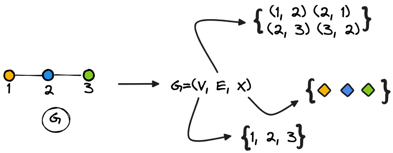
For this series, we will consider another dimension to describe graphs, which is associated with node features: our notation becomes G = (V, E, X), where X includes the numerical representation of the nodes characteristics. Figure 2 summarizes all these components (the colors are useful to represent the features):

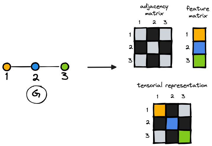
Figure 2 — Definition of a graph in terms of nodes, edges, and features

To feed GNN models, we can represent graphs in multiple ways, including the combination of an adjacency matrix that stores connectivity information and a feature matrix that describes the features of the nodes.

We can also merge these two representations using a tensor, in which the features are represented on the diagonal while the off-diagonal elements include information on the connectivity. Further details are reported in Figure 3.

Figure 3 — Representing graphs using matrices and tensors

Graph Isomorphism

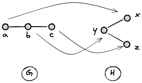
Graph isomorphism allows us to formally recognize in which cases two graphs have the same structures. To build an intuition about this concept, consider the following image, which depicts two graphs, G and H.

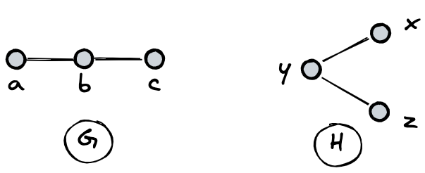
Are these two graphs, G and H, the same?

The answer to this question is no: nodes do not have the same labels. Moreover, G looks like a path, while H looks like a bipartite graph.

Do they have the same structure?

To answer this question, we will identify the main characteristics shared by distinct graphs with the same structure. Then, we will show how the definition of graph isomorphism is able to capture these characteristics.

Let’s build our intuitions on graph isomorphism

We assume that two graphs have the same structure if, in the first place, we can match each node of G to each node of H. Figure 5 clarifies this matching process, in which a is mapped to x, b is mapped to y, and c is mapped to z:

Figure 5 — Matching each single node of G to a single node of H

In the second place, matched nodes must play the same role in the two graphs. To clarify this point, let’s try depicting the nodes matched in the previous step with the same color. The result is shown in Figure 6.

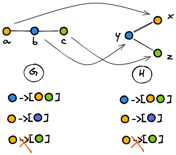
Figure 6— Connections (and non-connections) between matched nodes

Figure 6 clarifies how the corresponding nodes play the same role in the two graphs based on their connections (and non-connections) with the other nodes. In details:

The blue node has two neighbors: the yellow node and the green node.
The yellow node has one neighbor: the blue node.
The yellow and the green nodes are not neighbors.

To summarize, if two nodes are connected in graph G, then the corresponding nodes in graph H should be connected. On the other hand, if two nodes in G are not connected, then the corresponding nodes in H should not be connected.

A bit of formalism

The formal notion of isomorphism captures the informal idea that some objects have the same structure, ignoring individual distinctions of atomic components (the nodes, in our case). More specifically, the concept of graph isomorphism should be able to capture the two characteristics that we have introduced in the previous section:

The one-to-one mapping of the nodes between the two distinct graphs.
The perpetuation of the connections and non-connections of the corresponding nodes.

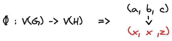
We can start to formalize this idea considering that two graphs are isomorphic if a function Φ takes the nodes (or vertices) from graph G and maps them to the nodes of graph H. Figure 7 reports the details of this function in our specific example.

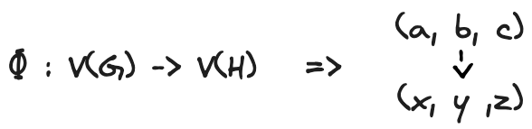
Figure 7— Details of Φ function mapping nodes between isomorphic graphs

The next step is to analyze the unique properties of the function Φ.

Firstly, as shown in Figure 8 and Figure 9, two nodes of G can not be mapped to the same node in H if we want to satisfy the idea of capturing the same structure in two distinct graphs.

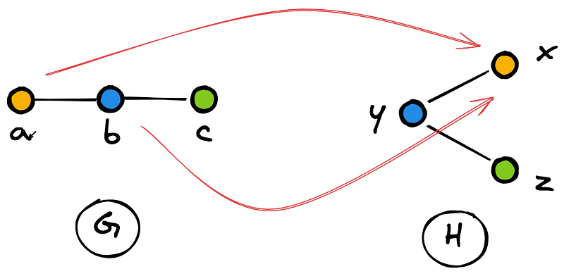
Figure 8— Two nodes of graph G (a,b) mapped to the same node in the graph H (x)

Figure 9— Φ mapping function formalizing the high-level idea expressed in Figure 5

To improve the intuitions, we can see the process from a different perspective: the function Φ should inform us on how to relabel the nodes of H to reconstruct graph G. Therefore, Φ has to map each distinct node of G to a different node of H. Considering this specific property, Φ is defined as an injective function. Below is the definition from Wikipedia:

[…] an injective function (also known as injection, or one-to-one function ) is a function f that maps distinct elements of its domain to distinct elements; that is, x1 ≠ x2 implies f(x1) ≠ f(x2). (Equivalently, f(x1) = f(x2) implies x1 = x2 in the equivalent contrapositive statement.)

Another crucial property of Φ is that every node of H has to be mapped to each node of G. If a node from H is not mapped to a node of G, then the two graphs do not have the same structure. This situation is described in Figure 10, in which all the nodes of G are mapped to some nodes of H, but the red node of H is not mapped to any node of G.

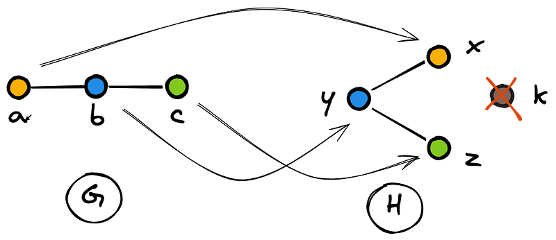
Figure 10— The k node has not a corresponding node in graph G

As clearly shown in Figure 10, H has one more node than G. Therefore, the two graphs can not have the same structure. The property according to which any node of H, or more broadly any element of the codomain, is getting mapped makes Φ a surjective function. Below is the definition of Wikipedia:

In mathematics, a surjective function (also known as surjection, or onto function /ˈɒn.tuː/) is a function f such that, for every element y of the function’s codomain, there exists at least one element x in the function’s domain such that f(x) = y. In other words, for a function f : X → Y, the codomain Y is the image of the function’s domain X.

Let’s understand how these two properties of Φ are complementary.

As we already mentioned, Φ should be an injective function: each node of G should be mapped to a distinct vertice of H. This property does not automatically guarantee that any node of H is mapped to G (Figure 7). For this reason, Φ should also be a surjective function: every node of H should be matched to any node of G. The surjectivity could allow Φ to map one or more elements of G to the same node of H. However, as shown in Figure 6, the injectivity property of Φ prevents this situation.

The combination of these two properties implies a one-to-one correspondence between the nodes of the two graphs, which makes Φ a bijective function. Below is the definition from Wikipedia:

A bijection, bijective function, or one-to-one correspondence between two mathematical sets is a function such that each element of the second set (the codomain) is mapped to from exactly one element of the first set (the domain). Equivalently, a bijection is a relation between two sets such that each element of either set is paired with exactly one element of the other set.

Finishing touches before coding

Our explanation focused on the node side of the graph.

But what about the edges?

In the introductory part related to the graph isomorphism problem, we also mentioned the crucial aspect of preserving the same connections (and the non-connections) between the matched nodes. More formally, our key goal is to maintain adjacencies and non-adjacencies in this mapping process.

Interestingly, we can describe this property by leveraging our Φ function, as shown in Figure 11.

Figure 11— Adjacencies and non-adjacencies preservation defined using the mapping function Φ

According to this expression, any pair of nodes of graph G should be connected by an edge if and only if their corresponding nodes (obtained by applying Φ) are also connected by an edge. Or, in other words, they are adjacent in the graph H.

Let’s gather all the ingredients involving nodes and edges in Figure 12.

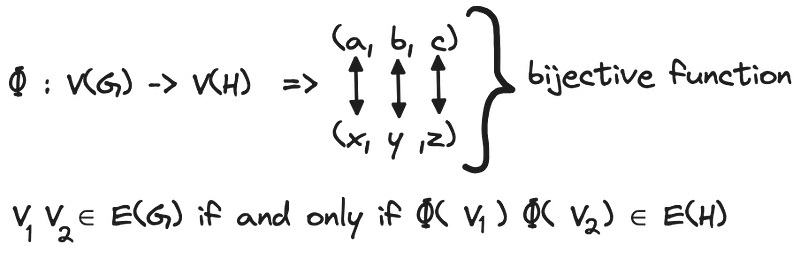
Figure 12— All the properties of the function Φ to make it an isomorphism

If a function Φ with the characteristics reported in Figure 12 exists, G and H are isomorphic graphs, and Φ is an isomorphism. Formally:

Two graphs, G and H, are isomorphic if there exists a bijection Φ:V(g) -> V(h) such that uv ∈ E(G) if and only if Φ(u) Φ(v) ∈ E(H). In this case, we can state: G≅H.

Graph Isomorphism Using Adjacency Matrices

In the previous section, we underlined that the concept of graph isomorphism implies the importance of maintaining adjacencies and non-adjacencies of the corresponding nodes. This suggests that the adjacency matrix we introduced at the beginning of this article has to play a crucial role.

To reason around this idea, let’s show explicitly the adjacency matrices of G and H, as shown in Figure 13.

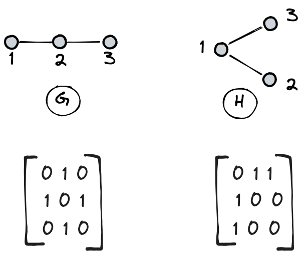
Figure 13 — G and H graphs relabeled using digits, and their related adjacency matrices

We relabeled our nodes using digits (1, 2, 3) by replacing our letters (a, b, c, or x, y, z) to simplify the matrix representation. This simple trick helps us leverage the digit label to identify the related row in the adjacency matrices.

From this example, it is clear that the two adjacency matrices are different, as well as our graphs G and H. Therefore, the key question is the following:

How can we define Φ as a matrix?

Let’s see how we can do it. Figure 14 recaps our mapping function using digits instead of letters.

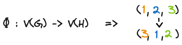
Figure 14 — Φ function using digits to label graph nodes

Figure 15 describes this mapping by leveraging a matrix:

Figure 15 — Matrix representing the mapping function Φ

The matrix reported in Figure 15 describes the mapping performed by Φ, from the nodes of G to the nodes of H. More specifically:

The 1st row of the matrix represents node 1 in G. The 3rd element of this row is initialized to 1. Therefore, node 1 of G is mapped to node 3 of H. The orange color describes this matching.
The 2nd row of the matrix represents node 2 in G. The 1st element of this row is initialized to 1. Therefore, node 2 of G is mapped to node 1 of H. The blue color describes this matching.
The 3rd row of the matrix represents node 3 in G. The 2nd element of this row is initialized to 1. Therefore, node 3 of G is mapped to node 2 of H. The green color describes this matching.

The matrix representing this transformation is also known as the Permutation matrix. According to Wikipedia:

[…] a permutation matrix is a square binary matrix that has exactly one entry of 1 in each row and each column with all other entries 0.[1] An n × n permutation matrix can represent a permutation of n elements.

We can describe the relationship between two isomorphic graphs in terms of adjacency and permutation matrices. This relationship is described in Figure 16.

Figure 16 — Definition of graph isomorphism in terms of adjacency and permutation matrices

According to the formula, a graph G is isomorphic to H if and only if there exists a permutation matrix P such that the adjacency matrix of G can be obtained by multiplying the permutation matrix P, the adjacency matrix of H, and the transpose of the permutation matrix P.

We can code our ingredients using NumPy to make our understanding more concrete. Firstly, we create the adjacency matrices of G and H and our permutation matrix P:

A_G = np.array([[0, 1, 0],  # Node 1
                [1, 0, 1],  # Node 2
                [0, 1, 0]]) # Node 3

A_H = np.array([[0, 1, 1],  # Node 1
                [1, 0, 0],  # Node 2
                [1, 0, 0]]) # Node 3

P = np.array([[0, 0, 1], # From Node 1 to Node 3
              [1, 0, 0], # From Node 2 to Node 1
              [0, 1, 0]]) # From Node 3 to Node 2

Let’s transpose the matrix P and compute the operations described in Figure 16.

P_t = np.transpose(P)

--- print(P_t)
array([[0, 1, 0],
       [0, 0, 1],
       [1, 0, 0]])
---

X = np.dot(np.dot(P, A_H), P_t)

--- print(X)
array([[0, 1, 0],
       [1, 0, 1],
       [0, 1, 0]])
---

np.array_equal(X, A_G)

--- print(np.array_equal(X, A_G))
true
---

Our simple code has shown that G is isomorphic to H and that this isomorphism has been described by means of the permutation matrix P and the adjacency matrices 𝐀𝓰 and Aₕ.

Conclusion

This article has shown how to define that the same structure characterizes two graphs. Such a definition, known as graph isomorphism, is fundamental for developing GNN models that are able to recognize these cases and provide the same representation of the two graphs. Or, even more important, to provide distinct representation in the case of non-isomorphic graphs.

In the next article of this series, we will take a step further and study the GNN architectures in terms of permutation equivariance and invariance. Comprehending these notions will allow us to analyze how GNNs work from this perspective and which principles we must follow to develop more powerful models.

References

If you are interested in reading more articles about the inner workings of Graph Neural Networks, you can read the following series about Graph Representation Learning: https://towardsdatascience.com/tagged/graphedm-series.

The author created all the images available in this article.