The Curse of Dimensionality, Demystified

Understanding the mathematical intuition behind the curse of dimensionality

The curse of dimensionality refers to the problems that arise when analyzing high-dimensional data. The dimensionality or dimension of a dataset refers to the number of linearly independent features in that dataset, so a high-dimensional dataset is a dataset with a large number of features. This term was first coined by Bellman in 1961 when he observed that the number of samples required to estimate an arbitrary function with a certain accuracy grows exponentially with respect to the number of parameters that the function takes.

In this article, we take a detailed look at the mathematical problems that arise when analyzing a high-dimensional set. Though these problems may look counterintuitive, it is possible to erxpalin them intuitively. Instead of a purely theoretical discussion, we use Python to create and analyze high-dimensional datasets and see how the curse of dimensionality manifests itself in practice. In this article, all images, unless otherwise noted, are by the author.

Dimension of a dataset

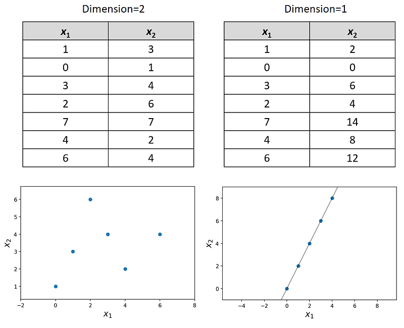
As mentioned before, the dimension of a dataset is defined as the number of linearly independent features that it has. A linearly independent feature cannot be written as a linear combination of the features in that dataset. Hence, if a feature or column in a dataset is a linear combination of some other features, it won’t add to the dimension of that dataset. For example, Figure 1 shows two datasets. The first one has two linearly independent columns and its dimension is 2. In the second dataset, one column is a multiple of another, hence we only have one independent feature. As the plot of this dataset shows, despite having two features, all the data points are along a 1-dimensional line. Hence the dimension of this dataset is one.

The effect of dimensionality on volume

The main reason for the curse of dimensionality is the effect of the dimension on volume. Here, we focus on the geometrical interpretation of a dataset. Generally, we can assume that a dataset is a random sample drawn from a population. For example, assume that our population is the set of points on a square shown in Figure 2. This square is the set of all points (x₁, x₂) such that 0≤x₁≤1 and 0≤x₂≤1, and the side length of this square is one.

Each population has its own distribution, and here we assume that the points on this square are uniformly distributed. It means that if we try to randomly select a point from this population, all the points have an equal chance of being selected. Now, if we draw a random sample of size n from this population (which means randomly selecting n points from this square), these points form a dataset with n rows and two features. So, the dimension of this dataset is 2.

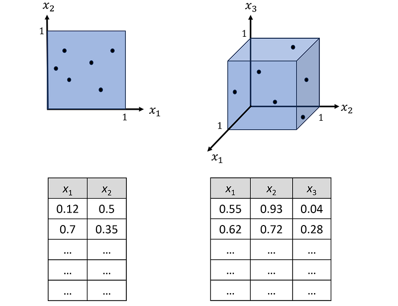
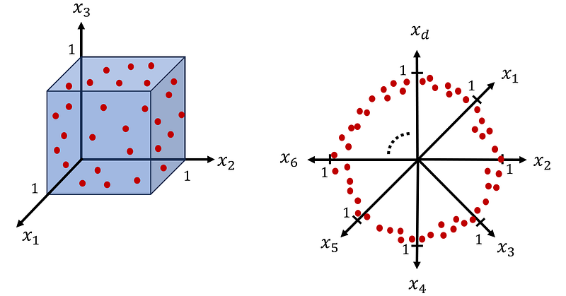
Similarly, we can create a dataset with a dimension of 3 by drawing a random sample from a cube of edge length 1 (Figure 2). This cube is the set of all points (x₁, x₂, x₃) such that 0≤x₁≤1, 0≤x₂≤1, and 0≤x₃≤1, and the points on this cube are uniformly distributed.

Finally, we can extend this idea and create a d-dimensional dataset by drawing a random sample of size n from a d-dimensional hypercube with an edge length of 1. The hypercube is defined as the set of all points (x₁, x₂,…, x_d) such that 0≤xᵢ≤1 (for i=1…d). Again, we can assume that the points in this hypercube are uniformly distributed. The resulting dataset has n examples (observations) and d features.

The volume of a d-dimensional hypercube with an edge length of L is L^d. (please note that if d=2, this formula gives the area of a square with a side length of L. However, here we assume that area is a special case of volume for a 2-dimensional object). Hence, if L=1, the volume is 1 no matter what the value of d is. But what is important is not the total volume of the hypercube, but how volume is distributed inside the hypercube. Here we use an example to explain it.

We can divide a unit square into 10 shells as shown in Figure 3. The first shell is indeed a small square at the center of the unit square and its edge length is 0.1. The bottom-right corner of this square is located at x₁=0.55. The bottom-right corner of the second shell is at x₁=0.6, so its thickness is 0.05. All the remaining shells have the same thickness and the bottom-right corner of the outermost shell is at x₁=1. Hence, it covers the sides of the unit square. Figure 3 shows one of these shells as an example whose bottom-right corner is at x₁=0.8.

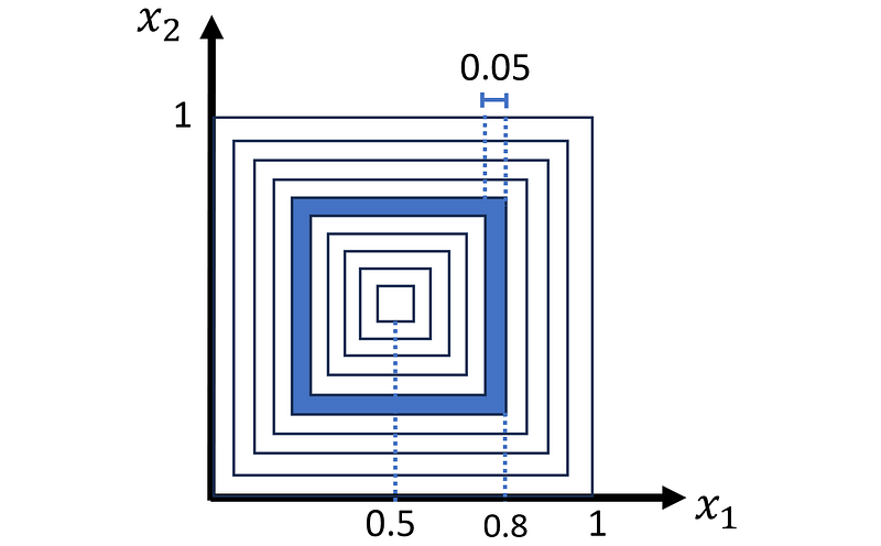
We can easily calculate the volume (area) of a shell whose bottom-right corner is located at x₁=c:

Now we can extend this procedure to a d-dimensional hypercube. We divide the hypercube into 10 hypercubic shells with the same thickness.

The volume of a shell with one of its corners at x₁=c is determined by the following formula:

Listing 1 calculates the volume of all these shells for different values of d and creates a bar plot of the volumes. The result is shown in Figure 4.

# listing 1

import numpy as np
import matplotlib.pyplot as plt
from scipy.stats import uniform, norm
from scipy.spatial import distance_matrix
from sklearn.neighbors import KNeighborsRegressor
%matplotlib inline

num_dims=[2, 3, 9, 15, 50, 100]
x_list = np.linspace(0.5, 1, 11)
edge_list = 2*(x_list - 0.5)
fig, axs = plt.subplots(3, 2, figsize=(14, 19))
plt.subplots_adjust(hspace=0.3)

for i, d in enumerate(num_dims):
    vols = [(edge_list[i+1])**d-(edge_list[i])**d \
            for i in range(len(x_list)-1)]
    axs[i//2, i%2].bar(x_list[1:], vols, width = 0.03)
    axs[i//2, i%2].set_title("d={}".format(d), fontsize=20)
    axs[i//2, i%2].set_xlabel('Shell corner $x_1$ coordinate', fontsize=18)
    axs[i//2, i%2].set_ylabel('Volume', fontsize=18)
    axs[i//2, i%2].set_xticks(x_list)
    axs[i//2, i%2].tick_params(axis='both', labelsize=12)

plt.show()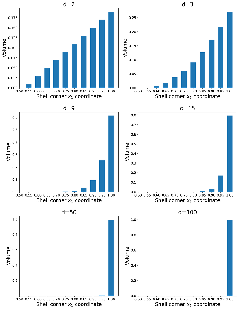

As you see as the number of dimensions increases, the share of the total volume for the inner shells decreases quickly. In fact, for d≥50, the outermost shell (whose corner is located at x₁=1) has more than 99% of the total volume of the unit hypercube. Hence, we conclude that in a high-dimensional hypercube, almost all of the volume is near the faces of the hypercube not inside it.

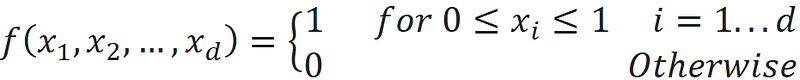
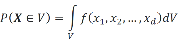
Now let’s calculate the probability of finding a data point in each shell. Remember that we assumed that the points in this hypercube are uniformly distributed. The probability that a random data point is within a certain shell can be calculated by integrating the probability density function (PDF) of the uniform distribution over the volume of that shell. The PDF of a continuous uniform distribution over a unit hypercube is:

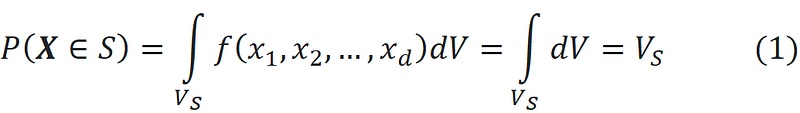
So the probability that a random data point lies within one of the shells (denoted by S) is simply equal to the volume of that shell:

Hence, based on the results of Figure 4, if we randomly sample a data point from the high-dimensional hypercube, there is a great chance that it will be in the outer shells. For d≥50, the probability of this random data point being in the inner shells is almost zero.

We can also confirm these results using Python. Listing 2 takes a sample of size 5000 from a uniform disitrubtion defined over a d-dimensional unit hypercube. Then it calculates the number of data points that belong to each shell and creates a bar plot of them. It uses the same values of d used in Listing 1.

# Listing 2

np.random.seed(0)
num_dims=[2,3,9, 15, 50, 100]
x_list = np.linspace(0.5, 1, 11)
x_list[-1] = 1.001
x_list1 = np.linspace(0.5, 0, 11)
x_list1[-1] = -0.001
fig, axs = plt.subplots(3, 2, figsize=(14, 19))
plt.subplots_adjust(hspace=0.3)

for i, d in enumerate(num_dims):
    sample = uniform.rvs(size=5000*d).reshape(5000, d)
    count_list=[]
    for j in range(len(x_list)-1):
        inshell_count = (((x_list[j] <= sample) & \
                          (sample < x_list[j+1])) | \
                          ((x_list1[j+1] < sample) & \
                          (sample <= x_list1[j]))).sum(axis=1)
        outshell_count = ((x_list[j+1] <= sample) | \
                          (x_list1[j+1] >= sample)).sum(axis=1)
        count = ((inshell_count>0) & (outshell_count==0)).sum()
        count_list.append(count)

    axs[i//2, i%2].bar(x_list[1:], count_list, width = 0.03)
    axs[i//2, i%2].set_title("d={}".format(d), fontsize=20)
    axs[i//2, i%2].set_xlabel('Shell corner $x_1$ coordinate', fontsize=18)
    if i%2==0:
        axs[i//2, i%2].set_ylabel('Number of data \npoints within shell',
                                  fontsize=18)
    axs[i//2, i%2].set_xticks(np.linspace(0.5, 1, 11))
    axs[i//2, i%2].tick_params(axis='both', labelsize=12)

plt.show()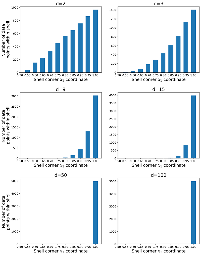

The plots are shown in Figure 5, and as you see the shape of the bar plots is similar to that of Figure 4. The number of data points in each shell is proportional to the corresponding probability of that shell given in Equation 1, so they are proportional to the volume of that shell. In fact, when d=100, almost all of the data points are contained within the outermost shell, and this is a manifestation of the curse of dimensionality.

In a high-dimensional hypercube, almost all the observations of a random sample are near the faces (Figure 6). If the hypercube is d-dimensional, these observations can also represent a dataset with d features. Such a dataset is clearly not representative of the population that it was sampled from. Here the population is the set of all the data points in the hypercube, but our sample only contains the data points near the faces of the hypercube. In practice, we have no data points from the regions which are closer to the center of the hypercube. Suppose that we use such a sample as a training data set for a machine-learning model. The model never sees a data point that is near the center of the hypercube during training, so its prediction for such a data point won’t be reliable. In fact, the model cannot generalize its prediction to such data points.

We can also find a different interpretation for these results. Suppose that we have uniform disitrubtion defined on the interval [0,1]. This is like a 1-dimensional space. If we take a random sample of size 1 from it and denote it by X₁, then we have:

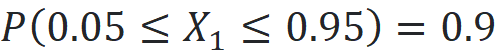
So, the probability that the X₁ is within 0.05 units of the interval’s edges is just 10%. Now suppose that we have a sample of size 1 from a 100-dimensional uniform distribution and denote it by X₁, X₂, … X₁₀₀. This is an IID (independent and identically distributed) sample which means that all Xᵢs are independent and each Xᵢ has uniform disitrubtion on the interval [0,1]. So, we can write:

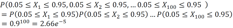
And we get:

As a result, the probability that at least one Xᵢ is within 0.05 units of one of the hypercube’s faces is almost 1 (and this means that the observation with that Xᵢ is within 0.05 units of that face). On average, in a sample of size 37594, we can find only one data point that is not in this region (1 / 2.66e-5 ≈ 37594). This means that we need a very large sample to get just a few data points that are not near the faces of the hypercube.

As the number of dimensions (or features) in a dataset increases, the amount of observations needed to generalize the machine learning model accurately increases exponentially. The curse of dimensionality makes the training data set sparse, and generalizing the model’s predictions becomes more difficult. Hence, we need much more training data (more observations) to generalize the model. In reality, preparing such a big training data set may be impractical.

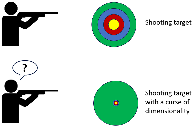
Figure 7 shows an analogy for the effect of the curse dimensionality on random sampling. Initially, we have a 2-dimensional shooting target and a novice shooter who randomly shoots at it. He has a chance of hitting the innermost ring. At the bottom, we have the same target which now has the curse of dimensionality. Almost all the targeting area belongs to the outermost ring, so the chance of hitting the innermost ring is almost zero.

The effect of the curse of dimensionality on random sampling is not limited to a uniform distribution. In fact, it happens for any high-dimensional dataset regardless of its probability disitrubtion. Let’s see what happens if the features in a dataset have a normal disitrubtion. Let’s assume that all the features in our dataset are independent and have a standard normal disitrubtion. As a result, if we combine these features in a vector, that vector has a standard multivariate normal distribution. Figure 8 shows the PDF of a 2-dimensional standard multivariate normal distribution.

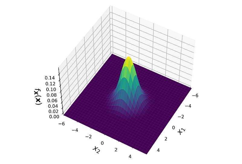
The PDF of the standard norma disitrubtion is the product of the PDF of its marginal distributions:

where each f(xᵢ) is the PDF of a standard normal disitrubtion. Using this equation we can plot the PDF of the standard normal disitrubtion at higher dimensions. Listing 3 plots the PDF of a d-dimensional standard normal disitrubtion for 3 values of d along one of the axes (xᵢ). Please note that the PDF has a symmetric shape, so the plot is the same for all xᵢ and for all lines that pass through the origin. Based on these plots, we conclude that the maximum value of the PDF is at the origin for any value of d, and it drops as we move away from the origin.

# Listing 3

np.random.seed(0)
num_dims=[2, 5, 10]
xi = np.linspace(-3, 3, 500)
fig, axs = plt.subplots(1, 3, figsize=(19, 5))
plt.subplots_adjust(wspace=0.25)

for i, d in enumerate(num_dims):
    pdf = norm.pdf(xi)**d
    axs[i].plot(xi, pdf)
    axs[i].set_xlabel('$x_i$', fontsize=28)
    axs[i].set_xlim([-3, 3])
    axs[i].set_title("d={}".format(d), fontsize=26)
    axs[i].tick_params(axis='both', labelsize=12)
axs[0].set_ylabel('PDF', fontsize=26)

plt.show()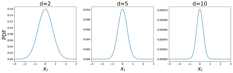

Listing 4 takes a sample of size 5000 from a d-dimensional standard multivariate normal distribution. Then it calculates the Euclidian distance of each d-dimensional data point in this sample from the origin. Finally, it creates a histogram of these distances. It uses the same values of d used in Listing 1. The result is shown in Figure 10.

# Listing 4

np.random.seed(0)
num_dims=[2,3,9, 15, 50, 100]
fig, axs = plt.subplots(2, 3, figsize=(19, 14))
plt.subplots_adjust(hspace=0.3)

for i, d in enumerate(num_dims):
    samples = norm.rvs(size=5000*d).reshape(5000, d)
    dist = np.linalg.norm(samples, axis=1)
    axs[i//3, i%3].hist(dist, bins=25)
    axs[i//3, i%3].set_title("d={}".format(d), fontsize=28)
    axs[i//3, i%3].set_xlabel('Distance from origin', fontsize=22)
    if i%3==0:
        axs[i//3, i%3].set_ylabel('Number of data points', fontsize=22)
    axs[i//3, i%3].set_xlim([0, 14])
    axs[i//3, i%3].tick_params(axis='both', labelsize=16)

plt.show()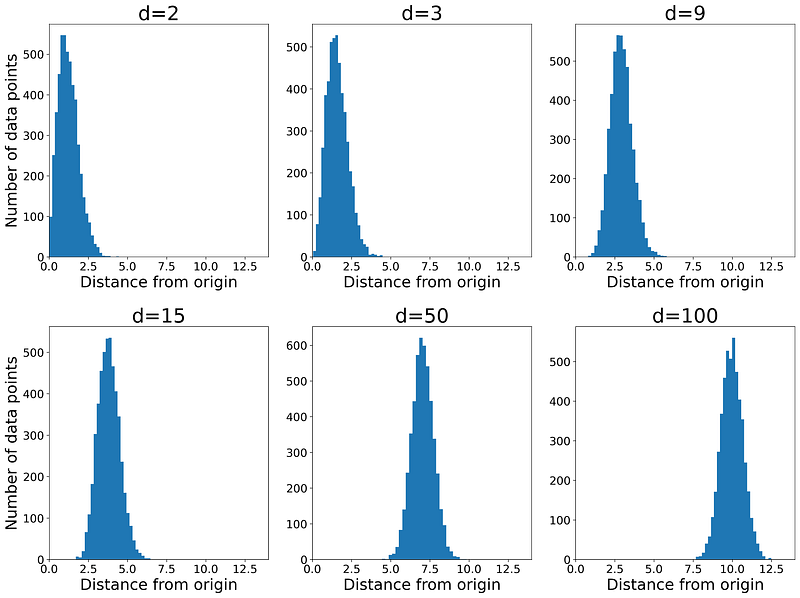

Here the number of data points in each bin of the histogram is proportional to the probability of finding a data point in that bin. As this figure shows, even when d=2, the peak of the histogram is not at zero. At the origin, the PDF has the maximum value (Figure 8), however, the probability also depends on the volume over which we take the integral:

By increasing the dimensionality, the peak of the radial histogram moves further from the origin. So the majority of the data points lie in a thin ring, and the probability of finding a point anywhere else is almost zero. Please note that the maximum value of the PDF is still at the origin at any value of d (Figure 9), however, the probability of obtaining a data point near the origin is almost zero. Again the dataset is not representative of the population that it was sampled from, and we have no data points from the regions that are very close to the origin and have a high PDF value.

It is important to note that the curse of dimensionality has nothing to do with the PDF of the probability disitrubtion of the dataset. For example, a uniform disitrubtion has the same value over its support no matter how many dimensions we have. However, since the probability depends on both the PDF and volume, it will be affected by the number of dimensions.

The effect of dimensionality on distance functions

The dimensionality also has an important effect on distance. First, let’s see what we mean by distance. Let x be a d-dimensional vector:

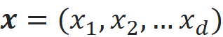
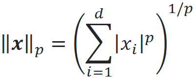
The p-norm of x is defined as:

We can calculate the distance between the vectors x and y using p-norms:

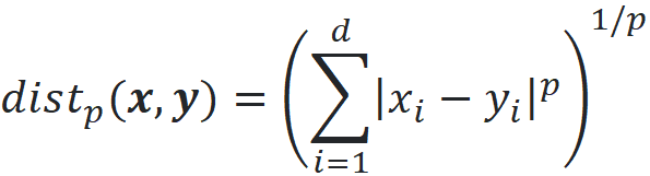
Please note that there are other types of distance functions, but in this article, we only focus on this type. When p=2, we get the familiar Euclidian distance:

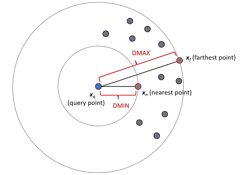
This is the length of the vector x-y which is also denoted by ||x-y|| (we can use a p-norm without a subscript when p=2). Now let’s see how dimensionality affects the distance function. Suppose that the dimensionality of our dataset is d. We pick one of the points in a data set as a query point and denote this point by the vector x_q. We find the nearest and farthest data points to the query point and denote them by the vectors x_n and x_f respectively (Figure 11). Then we calculate the distance between the query point and the nearest and farthest data points:

Now it can be shown that under certain reasonable assumptions on the data distribution, we have:

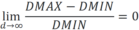
Hence, as dimensionality increases, the distance of the query point to the farthest data point approaches its distance to the nearest data point. Hence, differentiating the nearest data point from the other data points becomes impossible.

Listing 5 shows the effect of dimensionality on distance function. It draws a sample of size 500 from a uniform disitrubtion defined over a d-dimensional unit hypercube. Then it calculates the Euclidian distance between each pair of data points and plots a histogram of these distances. It uses the same values of d used in Listing 1. Figure 12 shows these histograms. Please note that in a d-dimensional unit hypercube, the minimum possible Euclidian distance between two points is zero and the maximum possible distance is:

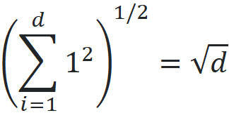
So, for each value of d, the limits of the x-axis of the histogram are 0 and √n.

# Listing 5

np.random.seed(0)
num_dims=[2,3,9, 15, 50, 500]
fig, axs = plt.subplots(2, 3, figsize=(19, 14))
plt.subplots_adjust(hspace=0.3)

for i, d in enumerate(num_dims):
    samples = uniform.rvs(size=500*d).reshape(500, d)
    dist_amtrix = distance_matrix(samples, samples)
    dist_arr = dist_amtrix[np.triu_indices(len(dist_amtrix), k = 1)]

    axs[i//3, i%3].hist(dist_arr, bins=30)
    axs[i//3, i%3].set_title("d={}".format(d), fontsize=28)
    axs[i//3, i%3].set_xlabel('Pairwise distance', fontsize=22)
    if i%3==0:
        axs[i//3, i%3].set_ylabel('Number of data points', fontsize=22)
    axs[i//3, i%3].set_xlim([0, np.sqrt(d)])
    axs[i//3, i%3].tick_params(axis='both', labelsize=16)

plt.show()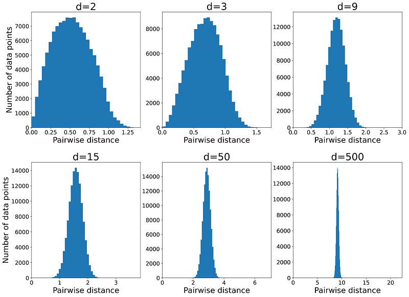

As the dimensionality (d) increases, the histogram becomes sharper, so all pairwise distances lie within a narrow range. This indicates that for each data point in the dataset, DMAX (the distance to the farthest data point) approaches DMIN (the distance to the nearest data point).

Let me explain the intuition behind this effect. Figure 13 shows a query point (x_q) and its nearest (x_n) and farthest data points (x_f). In a 2-dimensional space, each of the vectors

and

have 2 components. The components of x_n-x_q are marked in blue and those of x_f-x_q are marked in red. Similarly, in a d-dimensional space, these vectors have d components.

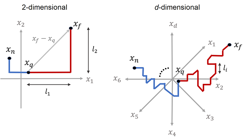
In a 2-dimensional space, to go from one point to another we should pass through 2 dimensions. For example, in Figure 13, to go from x_q to x_f, we should move l₁ units to the right and l₂ units up. Please note that l₁ and l₂ are the components of the vector x_f-x_q, and the distance between these points is the square root of l₁²+l₂². In a similar way, in a d-dimensional space, to go from x_q to x_f, we should pass through d dimensions. Now the vector x_f-x_q has d components. If the i-th component is denoted by lᵢ, then it means that we should move lᵢ units along the i-th dimension (Figure 13).

Listing 6 creates a sample of size 500 from a uniform disitrubtion defined over a d-dimensional unit hypercube. It then randomly picks a query data point (x_q) and finds its nearest (x_n) and farthest data point (x_f). Next, it calculates the components of the vectors x_n-x_q and x_f-x_q. Finally, the absolute values of these components are plotted in two bar plots for d=2 and d=500. The result is shown in Figure 14.

# Listing 6

np.random.seed(9)
num_dims=[2,500]
fig, axs = plt.subplots(2, 2, figsize=(17, 11))
plt.subplots_adjust(hspace=0.3)

for i, d in enumerate(num_dims):
    samples = uniform.rvs(size=500*d).reshape(500, d)
    query = samples[0]
    dist_amtrix = distance_matrix(samples, samples)
    ind_min = np.argmin(dist_amtrix[0, 1:])+1 
    ind_max = np.argmax(dist_amtrix[0, 1:])+1
    nearest = samples[ind_min]
    farthest = samples[ind_max]
    query_nearest_comps = np.abs(query - nearest)
    query_farthest_comps = np.abs(query - farthest)
    query_nearest_length = np.linalg.norm(query - nearest)
    query_farthest_length = np.linalg.norm(query - farthest)
    axs[0,i].bar(np.arange(1, d+1), query_nearest_comps,
               color="blue", width=0.45, label="$x_n-x_q$")
    axs[0,i].bar(np.arange(1, d+1), query_farthest_comps,
               color="red", alpha=0.5, width=0.45, label="$x_f-x_q$")
    axs[0,i].set_title("d={}".format(d), fontsize=26, pad=20)
    axs[0,i].set_xlabel('Index of component', fontsize=18)
    axs[0,i].set_ylabel('Abosulte value of component', fontsize=18)
    if i==0:
        axs[0,i].set_xticks(np.arange(1, d+1))
    axs[0,1].set_ylim([0, 1.2])
    axs[0,i].tick_params(axis='both', labelsize=16)
    axs[0,i].legend(loc='best', fontsize=17)
    axs[1,i].bar(["$||x_n-x_q||$", "$||x_f-x_q||$"],
                 [query_nearest_length, query_farthest_length],
                 width=0.2)
    axs[1,i].tick_params(axis='both', labelsize=22)
    axs[1,i].set_ylabel('Length', fontsize=18)

plt.show()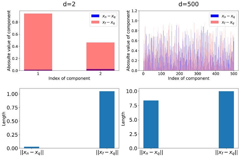

The length of the vector x_n-x_q gives the distance between x_q and x_n. Similarly, ||x_f-x_q|| gives the distance between x_q and x_f. These distances are also shown in separate bar plots in Figure 14. As this figure shows, in a 2-dimensional space, the absolute value of the components of x_n-x_q is much smaller than that of x_f-x_q. Hence the difference between ||x_f-x_q|| and ||x_n-x_q|| is noticable. In a 500-dimensional space, we have 500 components. As you see, the absolute value of some of the components of x_n-x_q is even greater than those of x_f-x_q. Remember that the length of a vector is obtained from the sum of the squares of these components. Hence, ||x_f-x_q|| and ||x_n-x_q|| are now much closer relatively.

We know that all the data points are chosen randomly, so the components of each data point are random numbers. When the dimensionality is high, to go from one point to another we should move through each dimension by a random distance (Figure 13), and since we have many dimensions, the total distance between each pair of points is roughly the same. Hence the distance from the query point to any other points is roughly the same. In fact, as the dimensionality increases, the average distance between the points increases, but the relative difference between these distances decreases (Figure 14).

Figure 15 gives an analogy for this effect. Assume that the path between two places is made up of several segments. In a 1-dimensional space, we only have one segment. In a 2-dimensional space, we have 2 segments between each pair of points, and in a d-dimensional space, we have d segments between them. When we only have one segment, the path length gives the actual horizontal distance between two points. Hence we can easily distinguish the closer point (n) from a further point (f).

As the number of segments increases, the path length (which is the sum of the length of all segments) increases and diverges from the actual distance between the points. Now the horizontal distance between the points doesn’t affect the path that much. Instead, the vertical movements along the segments determine the path length. As the number of segments goes to infinity, the length of the path between q and n approaches the length of the path between q and f.

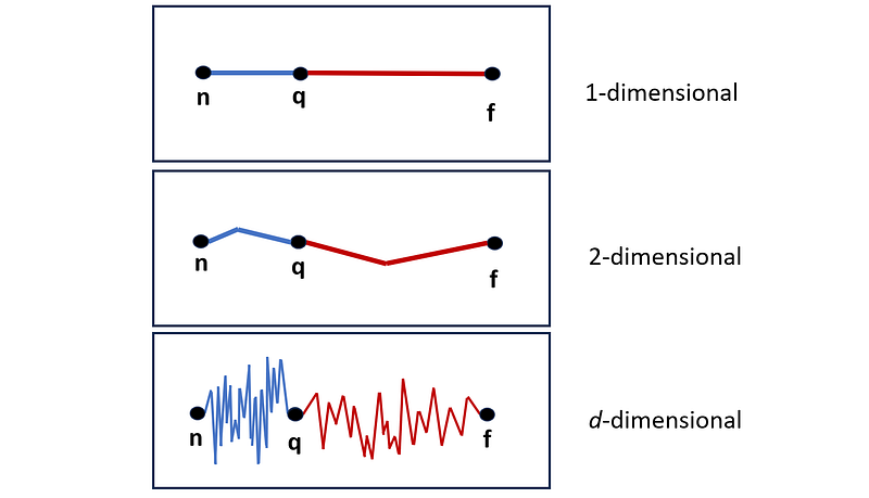
A path with d segments is similar to the distance between two points in a d-dimensional space, and each segment can represent one of the components of the vector that connects those points in that space. As dimensionality increases, we have more segments (components), and the relative difference between the distances approaches zero.

The effect of dimensionality on learning models

As mentioned in the previous section, in a high-dimensional space, the concept of proximity or distance is not meaningful anymore. Hence, any machine learning model that relies on the distance functions can break down in a high-dimensional space. In other words, when we have so many features in a training dataset, such models won’t give a reliable prediction anymore. One example is the k-NN (k Nearest Neighbors) algorithm. In this section, we will see how the curse of dimensionality affects the prediction error of a k-NN model (the examples are modified versions of those in [1]).

Our dataset has d features and 1000 examples (observations). These examples are drawn from a uniform disitrubtion over a unit d-dimensional hypercube. Hence each example of this dataset can be written as:

The target of this observation is defined as:

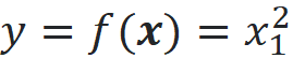
So, the target is simply the square of the first feature of each example. We use a k-NN model to predict the target for a test data point using this training dataset. To predict the target of a test data point, the k-NN model first finds the k nearest neighbors of that data point in the training data set (k nearest data point to the test point). It finds them using a distance function (Euclidian distance in this example). The predicted target of the test point is the average of the targets of these k nearest neighbors. In this example, we use the 3 nearest neighbors (k=3).

The test point is at the center of the hypercube:

We run 1000 simulations. In each simulation, we sample 1000 data points from a d-dimensional uniform distribution to create examples of the training dataset and calculate their target values. Then we train a k-NN model (with k=3) on this training dataset. Finally, we predict the target of the test data point (denoted by y^_t) using this model and compare it with the actual target which is 0.25. Once we have the predicted target for all the simulations, we can calculate the bias, variance, and mean squared error (MSE) of these predictions. Bias is defined as:

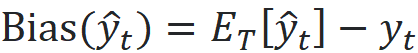
It is the difference between the mean of the predicted target (y^_t) over these simulations and the actual target of the test point (y_t). The variance is the variance of the predicted targets over these simulations:

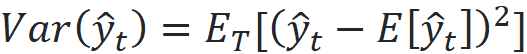
The mean squared error (MSE) is defined as:

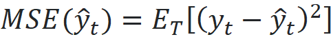
It can be shown that:

Listing 7 calculates the bias, variance, and MSE for this example for different values of d. The results are plotted in Figure 16.

# Listing 7

np.random.seed(2)
num_dims = np.arange(1, 11)
num_simulations = 1000

var_list = []
bias_list = []
for d in num_dims:
    pred_list = []
    for i in range(num_simulations):
        X = uniform.rvs(size=1000*d).reshape(1000, d)
        y = X[:,0]**2
        knn_model = KNeighborsRegressor(n_neighbors=3)
        knn_model.fit(X, y)
        pred_list.append(knn_model.predict(0.5*np.ones((1,d))))
    var_list.append(np.var(pred_list))
    bias_list.append((np.mean(pred_list)-0.25)**2)
error = np.array(bias_list) + np.array(var_list)
plt.plot(num_dims, var_list, 'o-', label="$Variance$")
plt.plot(num_dims, bias_list, 'o-', label="$Bias^2$")
plt.plot(num_dims, error, 'o-', label="$MSE$")
plt.xlabel("d", fontsize=16)
plt.ylabel("$MSE, Bias^2, Variance$", fontsize=16)
plt.legend(loc='best', fontsize=14)
plt.xticks(num_dims)
plt.show()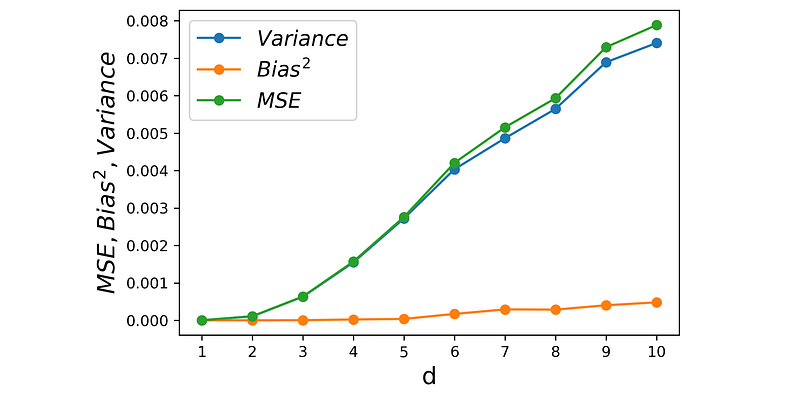

The k-NN model makes the assumption that close data points should also have close targets. However, in a high-dimensional dataset, all the data points are roughly at the same distance, so the k nearest neighbors can be very far from the test point. As a result, The average target of these neighbors is not an accurate prediction for the actual target of the test point anymore.

Listing 8 shows compares the k-NN prediction (y^_t) of all simulations for d=2 and d=10 (Figure 17). It also shows the actual target of the test point (y_t) with a black dashed line and the mean of all k-NN predictions with a blue line. Please note that the distance between the black dashed line and the blue line gives the bias.

# Listing 8

np.random.seed(2)
num_dims = [2, 10]
num_simulations = 1000
fig, axs = plt.subplots(1, 2, figsize=(10, 5))
plt.subplots_adjust(wspace=0.3)

for i, d in enumerate(num_dims):
    pred_list = []
    for j in range(num_simulations):
        X = uniform.rvs(size=1000*d).reshape(1000, d)
        y = X[:,0]**2
        knn_model = KNeighborsRegressor(n_neighbors=3)
        knn_model.fit(X, y)
        pred_list.append(knn_model.predict(0.5*np.ones((1,d))))
    axs[i].scatter([0]*num_simulations, pred_list,
                   color="blue", alpha=0.2, label="$\hat{y}_t$")
    axs[i].axhline(y = 0.25, color = 'black',
                   linestyle='--', label="$y_t$", linewidth=3)
    axs[i].axhline(y = np.mean(pred_list),
                   color = 'blue', label="$E[\hat{y}_t]$")
    axs[i].set_ylim([0, 0.7])
    axs[i].set_title("d={}".format(d), fontsize=18)
    axs[i].set_ylabel('$\hat{y}_t$', fontsize=18)
    axs[i].legend(loc='best', fontsize=14)
    axs[i].set_xticks([])

plt.show()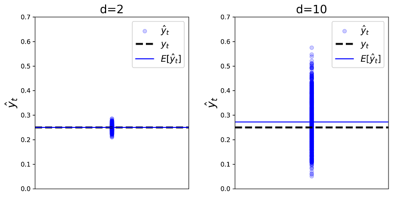

As dimensionality increases, the nearest neighbors will be near the faces of the hypercube, and very far from the test point at the center of the hypercube. The x₁ components of these points are not necessarily close to the x₁ of the test point and can vary a lot, hence the variance of the predictions quickly increases with d. However, on average they are close to x₁ of the test point, so the bias remains relatively small (Figure 16). The mean squared error (MSE) is proportional to both bias and variance, so it increases with dimensionality.

Listing 9 shows another example. Here the setup is similar to that of Listing 7, however, the target of the dataset is defined as:

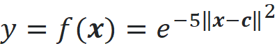
where

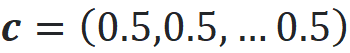
The test point is again at the center of the hypercube:

The plots of bias, variance, and MSE for this example are shown in Figure 18. Here the bias increases quickly with dimensionality and variance remains relatively small.

# Listing 9

np.random.seed(2)
num_dims = np.arange(1,11)
num_simulations = 1000

var_list = []
bias_list = []
for d in num_dims:
    pred_list = []
    for i in range(num_simulations):
        X = uniform.rvs(size=1000*d).reshape(1000, d)
        y = np.exp(-5*np.linalg.norm(X-0.5*np.ones((1,d)), axis=1)**2)
        knn_model = KNeighborsRegressor(n_neighbors=3)
        knn_model.fit(X, y)
        pred_list.append(knn_model.predict(0.5*np.ones((1,d))))
    var_list.append(np.var(pred_list))
    bias_list.append((np.mean(pred_list)-1)**2)
error = np.array(bias_list) + np.array(var_list)
plt.plot(num_dims, var_list, 'o-', label="$Variance$")
plt.plot(num_dims, bias_list, 'o-', label="$Bias^2$")
plt.plot(num_dims, error, 'o-', label="$MSE$")
plt.xlabel("d", fontsize=16)
plt.ylabel("$MSE, Bias^2, Variance$", fontsize=16)
plt.legend(loc='best', fontsize=14)
plt.xticks(num_dims)
plt.show()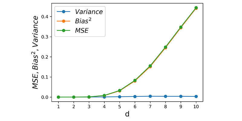

Remember that as dimensionality increases the distance between each pair of points increases but the relative difference between these distances approaches zero. Hence, for all data points including the the nearest neighbors, ||x|| increases and y goes to zero. So the average y^ of the nearest neighbors diverges from the target of the test point. The result is an increase in bias and MSE, but the variance remains small.

In summary, an increase in dimensionality increases MSE. However, its effect on bias or variance depends on how the target of the dataset is defined. These examples clearly show that k-NN is not a reliable model for high-dimensional data.

In this article, we discussed the curse of dimensionality and its effect on volume and distance functions. We saw that in a high-dimensional space, almost all of the data points will be far from the origin. Hence, if we use a high-dimensional dataset to train a model, the model’s prediction for a data point that is close to the origin won’t be reliable. In addition, the concept of distance is not meaningful anymore. In a high-dimensional dataset, the pairwise distance of all the data points is very close to each other. Hence the machine learning models that rely on distance functions won’t be able to give an accurate prediction for a high-dimensional dataset.

References

[1] Hastie, T., et al. The Elements of Statistical Learning. Springer, 2009.