Summary

The bias-variance tradeoff is a fundamental concept in machine learning that describes the balance between a model's ability to accurately fit the training data (low bias) and its ability to generalize to unseen data (low variance).

Abstract

The bias-variance tradeoff is a pivotal principle in the field of machine learning, encapsulating the challenge of creating models that are neither too simplistic nor too complex. A model with high bias tends to oversimplify the data, leading to underfitting and poor performance on both the training set and unseen data. Conversely, a model with high variance fits the training data very closely, capturing noise and specific patterns that do not generalize well to new data, resulting in overfitting. The tradeoff is quantified by the equation Prediction Error = Bias² + Variance + Noise, where the goal is to minimize the prediction error by finding an optimal balance between bias and variance. This balance is crucial for a model to perform well on unseen data, which is the ultimate test of its generalization ability.

Opinions

The article emphasizes that a model's complexity should be carefully managed to avoid underfitting or overfitting.
It is suggested that the true function generating the data is typically unknown and that the model's hypothesis should aim to approximate this function as closely as possible.
The noise in the data is acknowledged as an uncontrollable factor that contributes to the prediction error, highlighting the importance of focusing on minimizing bias and variance.
The article advocates for the use of techniques such as early stopping and regularization to manage the bias-variance tradeoff and improve model generalization.
There is an opinion that the ideal model should be complex enough to capture the underlying patterns in the data without being so complex that it fails to generalize to new data.

The Bias-Variance Tradeoff

The bias-variance tradeoff is an important concept in machine learning, which represents the tension that a model has between its ability to reduce the errors on the training set (its bias) versus its ability to generalize well to new unseen examples (its variance).

In general, as we make our model more complex (e.g., by adding more nodes to a decision tree), its bias decreases since the model adapts itself to the specific patterns and peculiarities of the training set (learning the training examples “by-heart”), and consequently the model loses its ability to generalize and provide good predictions on the test set (i.e., its variance increases).

Formal Analysis

The errors in a model’s predictions can be decomposed into three components:

Intrinsic noise in the data itself. This noise may be caused due to various reasons, such as internal noise in the physical devices that generated our measurements, or errors made by humans that entered the data into our databases.
The bias of the model, which represents the difference between the model’s predictions and the true labels of the data.
The variance of the model, which represents how the model’s predictions vary across different training sets.

In the following sections we are going to prove the following statement:

Prediction Error = Bias² + Variance + Noise

Typically, we cannot control the internal noise, but only the bias and the variance components of the prediction error. And since the prediction error of a given model is constant, trying to reduce its bias will increase its variance and vice versa (thereby we have the bias-variance tradeoff).

Definitions and Notations

Recall that in supervised machine learning problems, we are given a training set of n sample points, denoted by D = {(x₁, y₁), (x₂, y₂), … , (xₙ, yₙ)}, where xᵢ represents the features of point i (typically xᵢ is a vector) and yᵢ represents the true label of that point.

We assume that the labels are generated by some unknown function y = f(x) + ϵ, which our model is trying to learn. ϵ represents the intrinsic noise of the data, and we assume that it is uniformly distributed across all the data points with expected value of 0 (E[ϵ] = 0), and a standard deviation of σ (Var[ϵ] = σ²).

The function that our model learns from the given training set is called the model’s hypothesis and denoted by h(x).

Our goal is to find a hypothesis h(x) that is as close as possible to the true function f(x), or in other words, we would like to minimize the mean squared error between h(x) and the true labels y across all the possible data sets D that could have been used to train the model:

The subscript D is used to indicate that the model was built based on a specific training set D.

A model with a good generalization ability should give similar predictions regardless of the specific training set that was used to train it, since that would mean that the model has learned the general patterns in the data, rather than adapting itself to the specific peculiarities of the training set that was used to train it.

Formal Proof

Using our definition of y = f(x) + ϵ, we can write:

By rearranging the terms and expanding the square brackets we get:

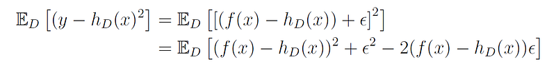
From the linearity of expectation we get:

The last term is equal to zero, since the expectation of the product of two variables is the product of the individual expectations, and the expectation of the noise is 0 ((E[ϵ] = 0). Therefore, we can write:

Since the noise ϵ does not depend on the specific training set D, and its variance is equal to σ², we can write:

We now make use of the fact that Var(X) = E[X²] - E[X]² to write:

And by rearranging the terms we get:

Since f(x) does not depend on the specific training set D, it does not affect the variance, thus we can write:

Substituting this expression back into the equation for the prediction error we get our final result:

The first term on the right side of this equation represents the bias squared, since E[f(x)-h(x)] is the expected error between the model’s predictions and the true function. The second term represents the variance of the model, and the third term represents the noise.

Therefore, we have shown that:

Prediction Error = Bias² + Variance + Noise

Finding the Right Balance

The ideal model has both low bias and low variance, i.e., it predicts well on the training set but also does not change much when it is fed new data. However, in practice we cannot achieve both of these objectives at the same time.

When the model is too simple (e.g., using a linear regression to model a non-linear function), it ignores useful information in the data set, and therefore it will have a high bias. In this case, we say that the model is underfitting the data.

When the model is too complex (e.g., using a complex neural network to model a simple linear function), it adapts itself to the specific training set and therefore has a high variance. In this case, we say that the model is overfitting the data.

Therefore, we should strive to find a model that lays in the sweet spot between overfitting and underfitting, i.e., a model that is not too simple nor too complex.

There are various ways to find such models, depending on the specific machine learning algorithm that you are using. For example, in iterative algorithms (such as gradient descent), we can track the performance of the algorithm on a held-out validation set, and once the validation error starts climbing we can stop the training (this technique is called early stopping).

Another way to control the tradeoff between the bias and variance is by using regularization. Regularization is a technique to prevent overfitting by penalizing complex models. The idea is to add a penalty term to the cost function of the model, such that it becomes dependent on two factors:

Cost(h) = Training Error(h) + λ Complexity(h)

λ is a hyperparameter that controls the tradeoff between the bias and the variance. Higher λ will induce a larger penalty on the complexity of the model, and thus will lead to simpler models with higher error on the training set but with smaller variance.

You can find more information about regularization in this article of mine.