The Art of Crossing Over Moving Averages in Python

Exploring different Moving Average Methods and Time Frame Variations for Strategic Advantage Optimization

Moving Averages are cornerstone concepts in technical analysis, yet their simplicity belies a deeper utility in trading. Moving averages, in their simplest form, serve as a tool to smooth out price data over a given time period, offering a glimpse into the underlying trend.

When these moving averages cross, they paint a picture that’s of significant interest to traders. A cross-over, is a moment where market sentiment is captured and a potential shift in market dynamics is signaled.

In Python, we quantify, test, and analyze, allowing traders and financial analysts to dissect and understand these pivotal points with great precision.

2. The Concept of Moving Average Cross-Overs

2.1 Basic Principle

When we talk about moving average cross-overs in the context of financial trading, we’re exploring a scenario where two trend lines — each representing the average price of an asset over different time frames — intersect.

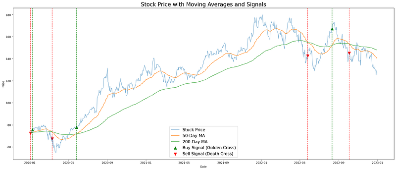
Imagine plotting a line that represents the average closing price of a stock over the last 50 days and another line for the last 200 days. Initially, these lines might follow a similar path, but at certain points, they cross each other.

2.2 Types of Cross-Overs

Golden Cross: The Golden Cross is a bullish signal traditionally seen when the shorter-term moving average, like the 50-day SMA, crosses above a longer-term moving average, like the 200-day SMA. It’s often interpreted as a signal that a new bullish trend is beginning.

Death Cross: In contrast, the Death Cross is a bearish signal. This occurs when the shorter-term moving average, such as the 50-day SMA, crosses below the longer-term moving average, like the 200-day SMA. Traders view this as a sign that a bearish trend could be starting.

2.3 Python Implementation

Implementing multiple moving average cross-overs in Python provides a hands-on way to explore and visualize these trading signals. Let’s dive into how you can do this effectively using different moving average methods and time-scales.

• Simple Moving Average (SMA): This is the average stock price over a specified number of days.
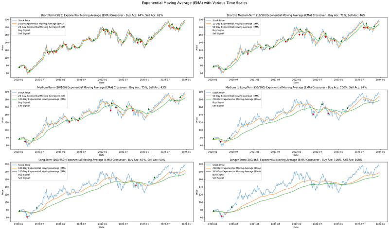
• Exponential Moving Average (EMA): EMA gives more weight to recent prices, making it more responsive to new information.
• Weighted Moving Average (WMA): WMA assigns a weighted multiplier to prices, emphasizing particular periods.

For more on Moving Average Methdologies, please read the following article(s). There are diverse methods that take volume and volatility into account.

2.3.1 Signal Identification

The core of our analysis is to identify when a short-term moving average crosses over a long-term moving average, signaling buy or sell opportunities.

This involves comparing the positions of the short-term and long-term averages: a crossover above signifies a buy (bullish trend), while a crossover below indicates a sell (bearish trend).

2.3.2 Accuracy Calculation

A unique aspect of our approach is the calculation of the accuracy of these signals. We look ahead a few days (in this case, five days) to see if the price moved in the direction indicated by the signal. This provides a practical measure of how reliable these signals have been historically.

2.3.3 Practical Insights

We analyze moving averages over various time scales, from short-term to longer-term, to understand how the effectiveness of these signals changes with time.

Furthermore, By plotting SMA, EMA, and WMA, we can compare how different types of moving averages behave in the same time frame and under the same market conditions.

import yfinance as yf
import matplotlib.pyplot as plt
import pandas as pd
import numpy as np

# Fetch stock data
def fetch_data(stock_symbol, start_date, end_date):
    data = yf.download(stock_symbol, start=start_date, end=end_date)
    return data

# SMA Function
def SMA(data, window):
    return data.rolling(window=window).mean()

# EMA Function
def EMA(data, window):
    return data.ewm(span=window, adjust=False).mean()

# WMA Function
def WMA(data, window):
    weights = np.arange(1, window + 1)
    return data.rolling(window=window).apply(lambda prices: np.dot(prices, weights[::-1])/weights.sum(), raw=True)

# Identify buy and sell signals
def identify_signals(data, short_window, long_window, ma_function):
    data['Short_MA'] = ma_function(data['Close'], short_window)
    data['Long_MA'] = ma_function(data['Close'], long_window)
    data['Signal'] = 0
    data['Signal'] = np.where(data['Short_MA'] > data['Long_MA'], 1.0, 0.0)
    data['Positions'] = data['Signal'].diff()
    return data

# Calculate accuracy
def calculate_accuracy(data):
    data['Future_Close'] = data['Close'].shift(-5)  # Looking 5 days ahead
    buys = data[(data['Positions'] == 1) & (data['Close'] < data['Future_Close'])]
    sells = data[(data['Positions'] == -1) & (data['Close'] > data['Future_Close'])]
    buy_accuracy = len(buys) / len(data[data['Positions'] == 1]) if len(data[data['Positions'] == 1]) > 0 else np.nan
    sell_accuracy = len(sells) / len(data[data['Positions'] == -1]) if len(data[data['Positions'] == -1]) > 0 else np.nan
    return buy_accuracy, sell_accuracy

# Plotting Function for Moving Averages with signals
def plot_ma_signals(stock_data, combinations, ma_function, ma_label):
    fig, axs = plt.subplots(3, 2, figsize=(25, 15))
    fig.suptitle(f'{ma_label} with Various Time Scales', fontsize=16)

    term_labels = {
        (5, 20): "Short-Term (5/20)",
        (10, 50): "Short to Medium-Term (10/50)",
        (20, 100): "Medium-Term (20/100)",
        (50, 200): "Medium to Long-Term (50/200)",
        (100, 250): "Long-Term (100/250)",
        (200, 365): "Longer-Term (200/365)"
    }

    for i, (short_window, long_window) in enumerate(combinations, 1):
        data = identify_signals(stock_data.copy(), short_window, long_window, ma_function)
        buy_accuracy, sell_accuracy = calculate_accuracy(data)
        term_label = term_labels.get((short_window, long_window), f"{short_window}/{long_window}")

        ax = axs[(i-1)//2, (i-1)%2]
        ax.plot(data.index, data['Close'], label='Stock Price', alpha=0.5)
        ax.plot(data.index, data['Short_MA'], label=f'{short_window}-Day {ma_label}', alpha=0.8)
        ax.plot(data.index, data['Long_MA'], label=f'{long_window}-Day {ma_label}', alpha=0.8)
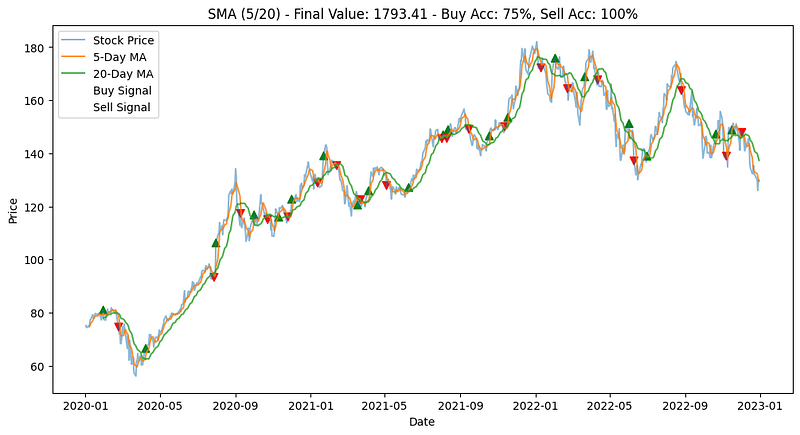
        ax.scatter(data.index, data['Close'], label='Buy Signal', marker='^', color='g', alpha=1, s=50 * data['Positions'].clip(lower=0))
        ax.scatter(data.index, data['Close'], label='Sell Signal', marker='v', color='r', alpha=1, s=50 * data['Positions'].clip(upper=0).abs())
        accuracy_title = f"Buy Acc: {buy_accuracy*100:.0f}%, Sell Acc: {sell_accuracy*100:.0f}%"
        ax.set_title(f'{term_label} {ma_label} Crossover - {accuracy_title}')
        ax.set_xlabel('Date')
        ax.set_ylabel('Price')
        ax.legend()

    plt.tight_layout(rect=[0, 0, 1, 0.96])
    plt.show()



# Main Functions Execution
stock = 'AAPL'
start_date = '2020-01-01'
end_date = '2024-01-01'
time_scale_combinations = [(5, 20), (10, 50), (20, 100), (50, 200), (100, 250), (200, 365)]

stock_data = fetch_data(stock, start_date, end_date)

# Plot for SMA
plot_ma_signals(stock_data, time_scale_combinations, SMA, "Simple Moving Average (SMA)")

# Plot for EMA
plot_ma_signals(stock_data, time_scale_combinations, EMA, "Exponential Moving Average (EMA)")

# Plot for WMA
plot_ma_signals(stock_data, time_scale_combinations, WMA, "Weighted Moving Average (WMA)")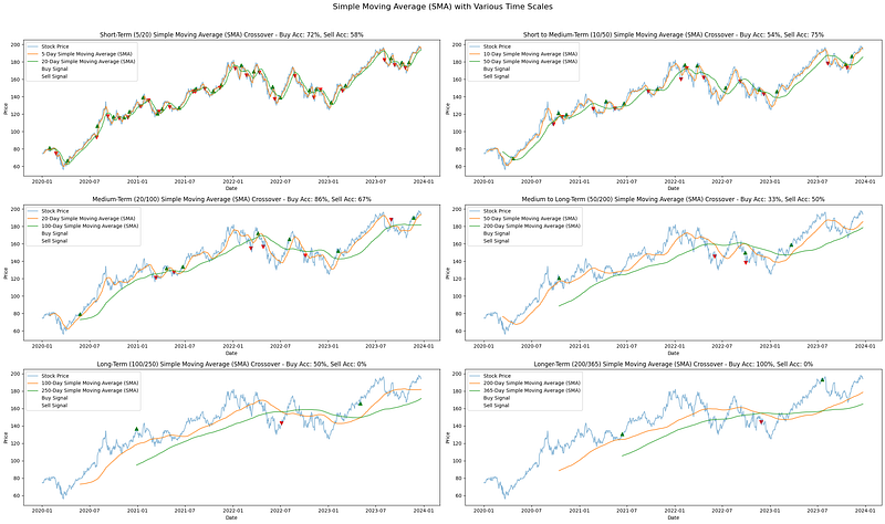

3. Analyzing Moving Average Cross-Overs

3.1 Interpreting Signals

The rational for interpreting the signals is as follows. A short-term moving average is more responsive to recent price changes compared to a long-term moving average.

When the short-term moving average crosses above the long-term average, it indicates that recent prices are consistently higher than the longer-term prices, suggesting an upward price trend.

Conversely, when the short-term average crosses below the long-term average, it shows that recent prices are lower, indicating a downward trend. These crossovers reflect shifts in market sentiment and momentum, influencing investor behavior and future price movements.

3.1 Different Time Frames

The effectiveness of moving average cross-overs can vary significantly across different time frames:

• Intraday vs. Long-Term: Intraday traders might use shorter time frames (like 5-day vs. 20-day MAs) for quick signals, while long-term investors might look at much longer periods (like 50-day vs. 200-day MAs).
• Impact on Strategy: Shorter time frames tend to produce more signals, but with potentially higher noise and false positives. Longer time frames provide fewer, but potentially more reliable, signals.

3.2 Best Practices

To enhance the effectiveness of moving average cross-over analysis:

• Consider Trading Volume: High trading volume can reinforce the strength of a cross-over signal. For instance, a Golden Cross with high trading volume might indicate strong buying interest.
• Use Multiple Time Frames for Confirmation: Relying on a single time frame can be risky. Using multiple time frames for confirmation can help in filtering out false signals. For example, if both short-term and long-term time frames indicate a bullish trend, the signal might be more reliable.

4. Optimizing Parameters

Optimizing parameters for moving average cross-overs involves testing various combinations of short-term and long-term windows to find the most effective strategy. This process can be quite extensive, but it’s essential for refining your trading approach.

The crux of the strategy lies in pinpointing the right moments to enter and exit the market. This step involves comparing the moving averages and discerning the cross-overs.

To measure the efficacy of the strategy, we would need to simulate trading scenarios and adjust the positions based on the identified signals and calculate the accuracy of these signals to ensure they align with market movements.

# Pseudocode to simulate trading
cash = 1000  # Initial cash
stock = 0    # Initial stock quantity
# Simulate the trading based on the 'Signal'...

Then experiment with different combinations of moving averages to determine the most effective.

Through rigorous testing of various time frames, identify which combination of short-term and long-term moving averages yields the best results.

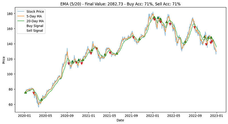
Finally plot the stock prices alongside the moving averages and signals to assess the strategy’s performance visually.

Visit www.entreprenerdly.com for the complete code and detailed explanation.

5. Limitations and Other Considerations

5.1 Limitations

Moving averages, while invaluable in trend analysis, come with inherent limitations that traders should be mindful of:

• Lagging Indicators: Since they are based on past data, moving averages inherently lag behind current market events. This delay can sometimes lead to late entry or exit signals in rapidly changing markets. There are various moving average methods that attempt to address this limitation.
• False Signals: Especially in sideways or choppy markets, moving averages can generate false signals, misleading traders about the strength or direction of a trend.

5.2 Mitigating Risks

To mitigate these risks, traders often combine moving averages with other indicators, like RSI or MACD, to confirm signals. It’s also advisable to analyze the overall market context and not rely solely on moving averages for decision-making.

5.3 Market Conditions

The effectiveness of moving average cross-overs can vary significantly under different market conditions:

• Volatile Markets: In highly volatile markets, moving averages might produce more false signals.
• Trending Markets: They tend to perform better in trending markets, where clear directional movements are present.

5.4 Strategy Adjustments

Adapting the strategy to current market conditions is crucial. For instance, in volatile markets, increasing the window size of the moving average can help filter out noise.

6. Concluding Thoughts

While the foundational aspects of moving average cross-overs are well-trodden, our approach, particularly through Python, brings a fresh perspective when optimizing and interpreting them within varied market contexts.

A promising area for further exploration is integrating machine learning with moving average strategies to enhance prediction accuracy and automate trading decisions.

Thank you for taking the time to read. If you found the article insightful, please consider clapping to support future content.👏