Getting Started

Text Classification Using Naive Bayes: Theory & A Working Example

In this article, I explain how the Naive Bayes works and I implement a multi-class text classification problem step-by-step in Python.

Table of contents

1. Introduction
2. The Naive Bayes algorithm
3. Dealing with text data
4. Working Example in Python (step-by-step guide)
5. Bonus: Having fun with the model
6. Conclusions

1. Introduction

Naive Bayes classifiers are a collection of classification algorithms based on Bayes’ Theorem. It is not a single algorithm but a family of algorithms where all of them share a common principle, i.e. every pair of features being classified is independent of each other.

Naive Bayes classifiers have been heavily used for text classification and text analysis machine learning problems.

Text Analysis is a major application field for machine learning algorithms. However the raw data, a sequence of symbols (i.e. strings) cannot be fed directly to the algorithms themselves as most of them expect numerical feature vectors with a fixed size rather than the raw text documents with variable length.

In this article I explain a) how Naive Bayes works, b) how we can use text data and fit them into a model after transforming them into a more appropriate form. Finally, I implement a multi-class text classification problem step-by-step in Python.

Let’s get started !!!

• NEW: After a great deal of hard work and staying behind the scenes for quite a while, we’re excited to now offer our expertise through a platform, the “Data Science Hub” on Patreon (https://www.patreon.com/TheDataScienceHub). This hub is our way of providing you with bespoke consulting services and comprehensive responses to all your inquiries, ranging from Machine Learning to strategic data analytics planning.
• Another resource. Learn Data Science and ML with the help of an 🤖 AI-powered tutor. Start here https://aigents.co/learn choose a topic and he will show up where you need him. No paywall, no signups, no ads.

2. The Naive Bayes algorithm

Naive Bayes classifiers are a collection of classification algorithms based on Bayes’ Theorem. It is not a single algorithm but a family of algorithms where all of them share a common principle, i.e. every pair of features being classified is independent of each other.

The dataset is divided into two parts, namely, feature matrix and the response/target vector.

• The Feature matrix (X) contains all the vectors(rows) of the dataset in which each vector consists of the value of dependent features. The number of features is d i.e. X = (x1,x2,x2, xd).
• The Response/target vector (y) contains the value of class/group variable for each row of feature matrix.

2.1. The main two assumptions of Naive Bayes

Naive Bayes assumes that each feature/variable of the same class makes an:

• independent
• equal

contribution to the outcome.

Side Note: The assumptions made by Naive Bayes are not generally correct in real-world situations. In-fact, the independence assumption is often not met and this is why it is called “Naive” i.e. because it assumes something that might not be true.

2.2. The Bayes’ Theorem

Bayes’ Theorem finds the probability of an event occurring given the probability of another event that has already occurred. Bayes’ theorem is stated mathematically as follows:

where:

• A and B are called events.
• P(A | B) is the probability of event A, given the event B is true (has occured). Event B is also termed as evidence.
• P(A) is the priori of A (the prior independent probability, i.e. probability of event before evidence is seen).
• P(B | A) is the probability of B given event A, i.e. probability of event B after evidence A is seen.

Summary

2.3. The Naive Bayes Model

Given a data matrix X and a target vector y, we state our problem as:

where, y is class variable and X is a dependent feature vector with dimension d i.e. X = (x1,x2,x2, xd), where d is the number of variables/features of the sample.

• P(y|X) is the probability of observing the class y given the sample X with X = (x1,x2,x2, xd), where d is the number of variables/features of the sample.

Now the “naïve” conditional independence assumptions come into play: assume that all features in X are mutually independent, conditional on the category y:

Finally, to find the probability of a given sample for all possible values of the class variable y, we just need to find the output with maximum probability:

3. Dealing with text data

One question that arises at this point is the following:

How are we going to use the raw text data to train the model ? The raw data is a collection of strings !

Text Analysis is a major application field for machine learning algorithms. However the raw data, a sequence of symbols (i.e. strings) cannot be fed directly to the algorithms themselves as most of them expect numerical feature vectors with a fixed size rather than the raw text documents with variable length.

In order to address this, scikit-learn provides utilities for the most common ways to extract numerical features from text content, namely:

• tokenizing strings and giving an integer id for each possible token, for instance by using white-spaces and punctuation as token separators.
• counting the occurrences of tokens in each document.

In this scheme, features and samples are defined as follows:

• each individual token occurrence frequency is treated as a feature.
• the vector of all the token frequencies for a given document is considered a multivariate sample.

“Counting” Example (to really understand this before we move on):

from sklearn.feature_extraction.text import CountVectorizer
corpus = [
    'This is the first document.',
    'This document is the second document.',
    'And this is the third one.',
    'Is this the first document?',
]

vectorizer = CountVectorizer()
X = vectorizer.fit_transform(corpus)

print(vectorizer.get_feature_names())
[‘and’, ‘document’, ‘first’, ‘is’, ‘one’, ‘second’, ‘the’, ‘third’, ‘this’]

print(X.toarray())
[[0 1 1 1 0 0 1 0 1]
 [0 2 0 1 0 1 1 0 1]
 [1 0 0 1 1 0 1 1 1]
 [0 1 1 1 0 0 1 0 1]]

In the above toy example, we have a collection of strings stored into the variable corpus. Using the text transformer, we can see that we have a specific number of unique strings (vocabulary) in our data.

This can be seen by printing the vectorizer.get_feature_names() variable. We observe that we have 9 unique words.

Next, we printed the transformed data (X) and we observe the following:

• We have 4 rows in X as the number of our text strings (we have the same number of samples after the transformation).
• We have the same number of columns (features/variables) in the transformed data (X) for all the samples (this was not the case before that transformation i.e. the individual strings had different lengths).
• The values 0,1,2, encode the frequency of a word that appeared in the initial text data.

E.g. The first transformed row is [0 1 1 1 0 0 1 0 1] and the unique vocabulary is [‘and’, ‘document’, ‘first’, ‘is’, ‘one’, ‘second’, ‘the’, ‘third’, ‘this’], thus this means that the words “document”, “first”, “is”, “the” and “this” appeared 1 time each in the initial text string (i.e. ‘This is the first document.’).

Side note: This is the counting approach. The term-frequency transform is nothing more than a transformation of a count matrix into a normalized term-frequency matrix.

Hope everything is clear now. If not, read this paragraph as many times as it is needed in order to really grasp the idea and understand this transformation. It is a fundamental step.

4. Working example in Python

Now that you understood how the Naive Bayes and the Text Transformation work, it’s time to start coding !

Problem Statement

As a working example, we will use some text data and we will build a Naive Bayes model to predict the categories of the texts. This is a multi-class (20 classes) text classification problem.

Let’s start (I will walk you through). First, we will load all the necessary libraries:

import numpy as np, pandas as pd
import seaborn as sns
import matplotlib.pyplot as plt
from sklearn.datasets import fetch_20newsgroups
from sklearn.feature_extraction.text import TfidfVectorizer
from sklearn.naive_bayes import MultinomialNB
from sklearn.pipeline import make_pipeline
from sklearn.metrics import confusion_matrix, accuracy_score

sns.set() # use seaborn plotting style

Next, let’s load the data (training and test sets):

# Load the dataset
data = fetch_20newsgroups()

# Get the text categories
text_categories = data.target_names

# define the training set
train_data = fetch_20newsgroups(subset="train", categories=text_categories)

# define the test set
test_data = fetch_20newsgroups(subset="test", categories=text_categories)

Let’s find out how many classes and samples we have:

print("We have {} unique classes".format(len(text_categories)))
print("We have {} training samples".format(len(train_data.data)))
print("We have {} test samples".format(len(test_data.data)))

The above prints:

We have 20 unique classes
We have 11314 training samples
We have 7532 test samples

So, this is a 20-class text classification problem with n_train = 11314 training samples (text sentences) and n_test = 7532 test samples (text sentences).

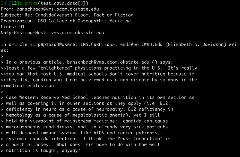
Let’s visualize the 5th training sample:

# let’s have a look as some training data
print(test_data.data[5])

As mentioned previously, our data are texts (more specifically, emails) so you should see something like the following printed out:

The next step consists of building the Naive Bayes classifier and finally training the model. In our example, we will convert the collection of text documents (train and test sets) into a matrix of token counts (I explained how this works in Section 3).

To implement that text transformation we will use the make_pipeline function. This will internally transform the text data and then the model will be fitted using the transformed data.

# Build the model
model = make_pipeline(TfidfVectorizer(), MultinomialNB())

# Train the model using the training data
model.fit(train_data.data, train_data.target)

# Predict the categories of the test data
predicted_categories = model.predict(test_data.data)

The last line of code predicts the labels of the test set.

Let’s see the predicted categories names:

print(np.array(test_data.target_names)[predicted_categories])
array(['rec.autos', 'sci.crypt', 'alt.atheism', ..., 'rec.sport.baseball', 'comp.sys.ibm.pc.hardware', 'soc.religion.christian'], dtype='<U24')

Finally, let’s build the multi-class confusion matrix to see if the model is good or if the model predicts correctly only specific text categories.

# plot the confusion matrix
mat = confusion_matrix(test_data.target, predicted_categories)
sns.heatmap(mat.T, square = True, annot=True, fmt = "d", xticklabels=train_data.target_names,yticklabels=train_data.target_names)
plt.xlabel("true labels")
plt.ylabel("predicted label")
plt.show()

print("The accuracy is {}".format(accuracy_score(test_data.target, predicted_categories)))

The accuracy is 0.7738980350504514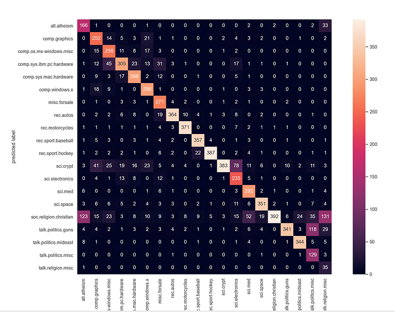

Note: If you’re passionate about diving deeper into machine learning with Python and sklearn, I highly recommend checking out this book; it’s a game-changer in breaking down complex topics into digestible insights.

5. Bonus: Having fun with the model

Let’s have some fun using the trained model. Let’s classify whatever sentence we like 😄.

# custom function to have fun
def my_predictions(my_sentence, model):
    all_categories_names = np.array(data.target_names)
    prediction = model.predict([my_sentence])
    return all_categories_names[prediction]

my_sentence = “jesus”
print(my_predictions(my_sentence, model))
['soc.religion.christian']

my_sentence = "Are you an atheist?"
print(my_predictions(my_sentence, model))
['alt.atheism']

We inserted the string “jesus” to the model and it predicted the class “[‘soc.religion.christian’]”.

Change the “my_sentence” into other stings and play with the model 😃.

6. Conclusions

We saw that Naive Bayes is a very powerful algorithm for multi-class text classification problems.

Side Note: If you want to know more about the confusion matrix (and the ROC curve) read this:

Interpreting the confusion matrix

From the above confusion matrix, we can verify that the model is really good.

• It is able to correctly predict all 20 classes of the text data (most values are on the diagonal and few are off-the-diagonal).
• We also notice that the highest miss-classification (value off-the-diagonal) is 131 (5 lines from the end, last column at the right). The value 131 means that 131 documents that belonged to the “religion miscellaneous ” category were miss-classified as belonging to the “religion christian” category.

Interesting thing that these 2 categories are really similar and actually one could characterize these as 2 subgroups of a larger group e.g. “religion” in general.

Finally, the accuracy on the test set is 0.7739 which is quite good for a 20-class text classification problem 🚀.

That’s all folks! Hope you liked this article.

If you liked and found this article useful, follow 👣 me to be able to see all my new posts.

Questions? Post them as a comment and I will reply as soon as possible.

My Profile (have a look to find out about my collection of articles):

Get in touch with me

• LinkedIn: https://www.linkedin.com/in/serafeim-loukas/

You may also like: