Text Analysis & Feature Engineering with NLP

Language Detection, Text Cleaning, Measures of Length, Sentiment Analysis, Named-Entity Recognition, N-grams Frequency, Word Vectors, Topic Modeling

Summary

In this article, using NLP and Python, I will explain how to analyze text data and extract features for your machine learning model.

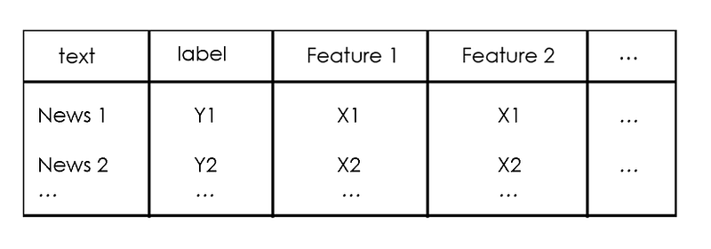
NLP (Natural Language Processing) is a field of artificial intelligence that studies the interactions between computers and human languages, in particular how to program computers to process and analyze large amounts of natural language data. NLP is often applied for classifying text data. Text classification is the problem of assigning categories to text data according to its content. The most important part of text classification is feature engineering: the process of creating features for a machine learning model from raw text data.

In this article, I will explain different methods to analyze text and extract features that can be used to build a classification model. I will present some useful Python code that can be easily applied in other similar cases (just copy, paste, run) and walk through every line of code with comments so that you can replicate this example (link to the full code below).

I will use the “News category dataset” (link below) in which you are provided with news headlines from the year 2012 to 2018 obtained from HuffPost and you are asked to classify them with the right category.

In particular, I will go through:

• Environment setup: import packages and read data.
• Language detection: understand which natural language data is in.
• Text preprocessing: text cleaning and transformation.
• Length analysis: measured with different metrics.
• Sentiment analysis: determine whether a text is positive or negative.
• Named-Entity recognition: tag text with pre-defined categories such as person names, organizations, locations.
• Word frequency: find the most important n-grams.
• Word vectors: transform a word into numbers.
• Topic modeling: extract the main topics from corpus.

Setup

First of all, I need to import the following libraries.

## for data
import pandas as pd
import collections
import json

## for plotting
import matplotlib.pyplot as plt
import seaborn as sns
import wordcloud

## for text processing
import re
import nltk

## for language detection
import langdetect 

## for sentiment
from textblob import TextBlob

## for ner
import spacy

## for vectorizer
from sklearn import feature_extraction, manifold

## for word embedding
import gensim.downloader as gensim_api

## for topic modeling
import gensim

The dataset is contained into a json file, so I will first read it into a list of dictionaries with the json package and then transform it into a pandas Dataframe.

lst_dics = []
with open('data.json', mode='r', errors='ignore') as json_file:
    for dic in json_file:
        lst_dics.append( json.loads(dic) )

## print the first one      
lst_dics[0]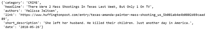

The original dataset contains over 30 categories, but for the purposes of this tutorial, I will work with a subset of 3: Entertainment, Politics, and Tech.

## create dtf
dtf = pd.DataFrame(lst_dics)

## filter categories
dtf = dtf[ dtf["category"].isin(['ENTERTAINMENT','POLITICS','TECH']) ][["category","headline"]]

## rename columns
dtf = dtf.rename(columns={"category":"y", "headline":"text"})

## print 5 random rows
dtf.sample(5)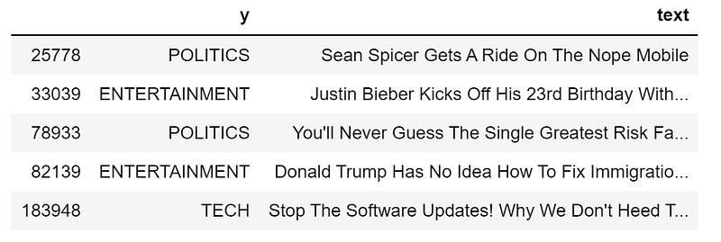

In order to understand the composition of the dataset, I am going to look into univariate distributions (probability distribution of just one variable) by showing labels frequency with a bar plot.

x = "y"

fig, ax = plt.subplots()
fig.suptitle(x, fontsize=12)
dtf[x].reset_index().groupby(x).count().sort_values(by= 
       "index").plot(kind="barh", legend=False, 
        ax=ax).grid(axis='x')
plt.show()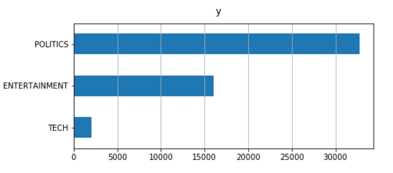

The dataset is imbalanced: the proportion of Tech news is really small compared to the others. This can be an issue during modeling and a resample of the dataset may be useful.

Now that it’s all set, I will start by cleaning data, then I will extract different insights from raw text and add them as new columns of the dataframe. This new information can be used as potential features for a classification model.

Let’s get started, shall we?

Language Detection

First of all, I want to make sure that I’m dealing with the same language and with the langdetect package this is really easy. To give an illustration, I will use it on the first news headline of the dataset:

txt = dtf["text"].iloc[0]

print(txt, " --> ", langdetect.detect(txt))

Let’s do it for the whole dataset by adding a column with the language information:

dtf['lang'] = dtf["text"].apply(lambda x: langdetect.detect(x) if 
                                 x.strip() != "" else "")

dtf.head()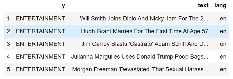

The dataframe has now a new column. Using the same code from before, I can see how many different languages there are:

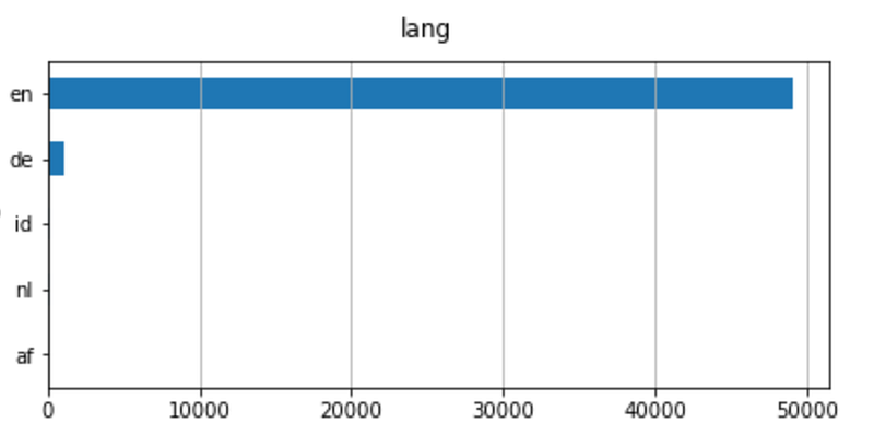
Even if there are different languages, English is the main one. Therefore I am going to filter the news in English.

dtf = dtf[dtf["lang"]=="en"]

Text Preprocessing

Data preprocessing is the phase of preparing raw data to make it suitable for a machine learning model. For NLP, that includes text cleaning, stopwords removal, stemming and lemmatization.

Text cleaning steps vary according to the type of data and the required task. Generally, the string is converted to lowercase and punctuation is removed before text gets tokenized. Tokenization is the process of splitting a string into a list of strings (or “tokens”).

Let’s use the first news headline again as an example:

print("--- original ---")
print(txt)

print("--- cleaning ---")
txt = re.sub(r'[^\w\s]', '', str(txt).lower().strip())
print(txt)

print("--- tokenization ---")
txt = txt.split()
print(txt)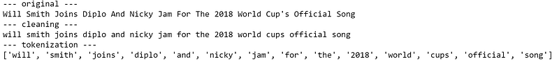

Do we want to keep all the tokens in the list? We don't. In fact, we want to remove all the words that don’t provide additional information. In the example, the most important word is “song” because it can point any classification model in the right direction. By contrast, words like “and”, “for”, “the” aren’t useful as they probably appear in almost every observation in the dataset. Those are examples of stop words. This expression usually refers to the most common words in a language, but there is no single universal list of stop words.

We can create a list of generic stop words for the English vocabulary with NLTK (the Natural Language Toolkit), which is a suite of libraries and programs for symbolic and statistical natural language processing.

lst_stopwords = nltk.corpus.stopwords.words("english")
lst_stopwords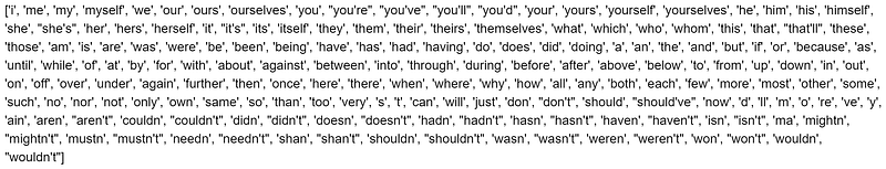

Let’s remove those stop words from the first news headline:

print("--- remove stopwords ---")
txt = [word for word in txt if word not in lst_stopwords]
print(txt)

We need to be very careful with stop words because if you remove the wrong token you may lose important information. For example, the word “will” was removed and we lost the information that the person is Will Smith. With this in mind, it can be useful to do some manual modification to the raw text before removing stop words (for example, replacing “Will Smith” with “Will_Smith”).

Now that we have all the useful tokens, we can apply word transformations. Stemming and Lemmatization both generate the root form of words. The difference is that stem might not be an actual word whereas lemma is an actual language word (also stemming is usually faster). Those algorithms are both provided by NLTK.

Continuing the example:

print("--- stemming ---")
ps = nltk.stem.porter.PorterStemmer()
print([ps.stem(word) for word in txt])

print("--- lemmatisation ---")
lem = nltk.stem.wordnet.WordNetLemmatizer()
print([lem.lemmatize(word) for word in txt])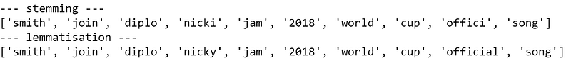

As you can see, some words have changed: “joins” turned into its root form “join”, just like “cups”. On the other hand, “official” only changed with stemming into the stem “offici” which isn’t a word, created by removing the suffix “-al”.

I will put all those preprocessing steps into a single function and apply it to the whole dataset.

'''
Preprocess a string.
:parameter
    :param text: string - name of column containing text
    :param lst_stopwords: list - list of stopwords to remove
    :param flg_stemm: bool - whether stemming is to be applied
    :param flg_lemm: bool - whether lemmitisation is to be applied
:return
    cleaned text
'''
def utils_preprocess_text(text, flg_stemm=False, flg_lemm=True, lst_stopwords=None):
    ## clean (convert to lowercase and remove punctuations and characters and then strip)
    text = re.sub(r'[^\w\s]', '', str(text).lower().strip())
            
    ## Tokenize (convert from string to list)
    lst_text = text.split()

    ## remove Stopwords
    if lst_stopwords is not None:
        lst_text = [word for word in lst_text if word not in 
                    lst_stopwords]
                
    ## Stemming (remove -ing, -ly, ...)
    if flg_stemm == True:
        ps = nltk.stem.porter.PorterStemmer()
        lst_text = [ps.stem(word) for word in lst_text]
                
    ## Lemmatisation (convert the word into root word)
    if flg_lemm == True:
        lem = nltk.stem.wordnet.WordNetLemmatizer()
        lst_text = [lem.lemmatize(word) for word in lst_text]
            
    ## back to string from list
    text = " ".join(lst_text)
    return text

Please note that you shouldn't apply both stemming and lemmatization. Here I am going to use the latter.

dtf["text_clean"] = dtf["text"].apply(lambda x: utils_preprocess_text(x, flg_stemm=False, flg_lemm=True, lst_stopwords))

Just like before, I created a new column:

dtf.head()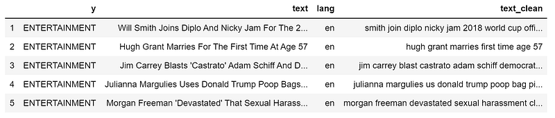

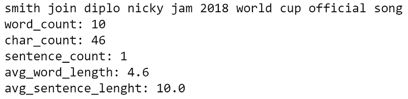
print(dtf["text"].iloc[0], " --> ", dtf["text_clean"].iloc[0])

Length Analysis

It’s important to have a look at the length of the text because it’s an easy calculation that can give a lot of insights. Maybe, for instance, we are lucky enough to discover that one category is systematically longer than another and the length would simply be the only feature needed to build the model. Unfortunately, this won’t be the case as news headlines have similar lengths, but it’s worth a try.

There are several length measures for text data. I will give some examples:

• word count: counts the number of tokens in the text (separated by a space)
• character count: sum the number of characters of each token
• sentence count: count the number of sentences (separated by a period)
• average word length: sum of words length divided by the number of words (character count/word count)
• average sentence length: sum of sentences length divided by the number of sentences (word count/sentence count)

dtf['word_count'] = dtf["text"].apply(lambda x: len(str(x).split(" ")))

dtf['char_count'] = dtf["text"].apply(lambda x: sum(len(word) for word in str(x).split(" ")))

dtf['sentence_count'] = dtf["text"].apply(lambda x: len(str(x).split(".")))

dtf['avg_word_length'] = dtf['char_count'] / dtf['word_count']

dtf['avg_sentence_lenght'] = dtf['word_count'] / dtf['sentence_count']

dtf.head()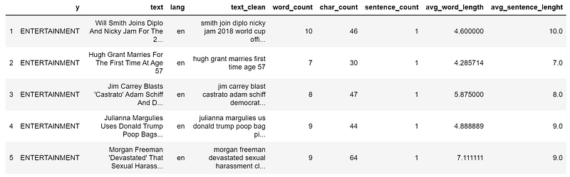

Let’s see our usual example:

What’s the distribution of those new variables with respect to the target? To answer that I’ll look at the bivariate distributions (how two variables move together). First, I shall split the whole set of observations into 3 samples (Politics, Entertainment, Tech), then compare the histograms and densities of the samples. If the distributions are different then the variable is predictive because the 3 groups have different patterns.

For instance, let’s see if the character count is correlated with the target variable:

x, y = "char_count", "y"

fig, ax = plt.subplots(nrows=1, ncols=2)
fig.suptitle(x, fontsize=12)
for i in dtf[y].unique():
    sns.distplot(dtf[dtf[y]==i][x], hist=True, kde=False, 
                 bins=10, hist_kws={"alpha":0.8}, 
                 axlabel="histogram", ax=ax[0])
    sns.distplot(dtf[dtf[y]==i][x], hist=False, kde=True, 
                 kde_kws={"shade":True}, axlabel="density",   
                 ax=ax[1])
ax[0].grid(True)
ax[0].legend(dtf[y].unique())
ax[1].grid(True)
plt.show()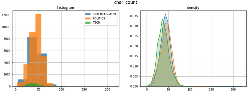

The 3 categories have a similar length distribution. Here, the density plot is very useful because the samples have different sizes.

Sentiment Analysis

Sentiment analysis is the representation of subjective emotions of text data through numbers or classes. Calculating sentiment is one of the toughest tasks of NLP as natural language is full of ambiguity. For example, the phrase “This is so bad that it’s good” has more than one interpretation. A model could assign a positive signal to the word “good” and a negative one to the word “bad”, resulting in a neutral sentiment. That happens because the context is unknown.

The best approach would be training your own sentiment model that fits your data properly. When there is no enough time or data for that, one can use pre-trained models, like Textblob and Vader. Textblob, built on top of NLTK, is one of the most popular, it can assign polarity to words and estimate the sentiment of the whole text as an average. On the other hand, Vader (Valence aware dictionary and sentiment reasoner) is a rule-based model that works particularly well on social media data.

I am going to add a sentiment feature with Textblob:

dtf["sentiment"] = dtf[column].apply(lambda x: 
                   TextBlob(x).sentiment.polarity)
dtf.head()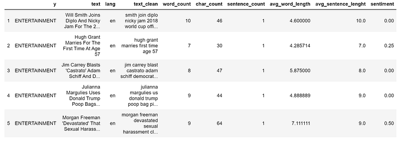

print(dtf["text"].iloc[0], " --> ", dtf["sentiment"].iloc[0])

Is there a pattern between categories and sentiment?

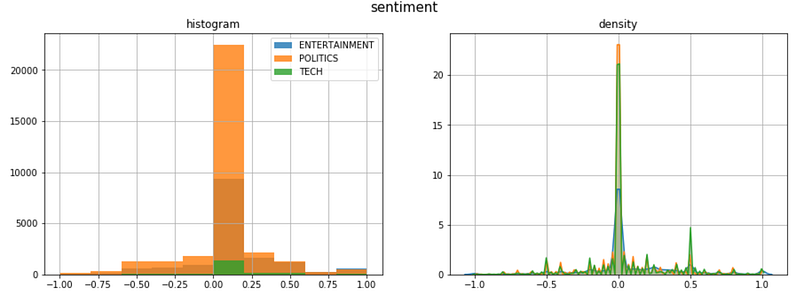
Most of the headlines have a neutral sentiment, except for Politics news that is skewed on the negative tail, and Tech news that has a spike on the positive tail.

Named-Entity Recognition

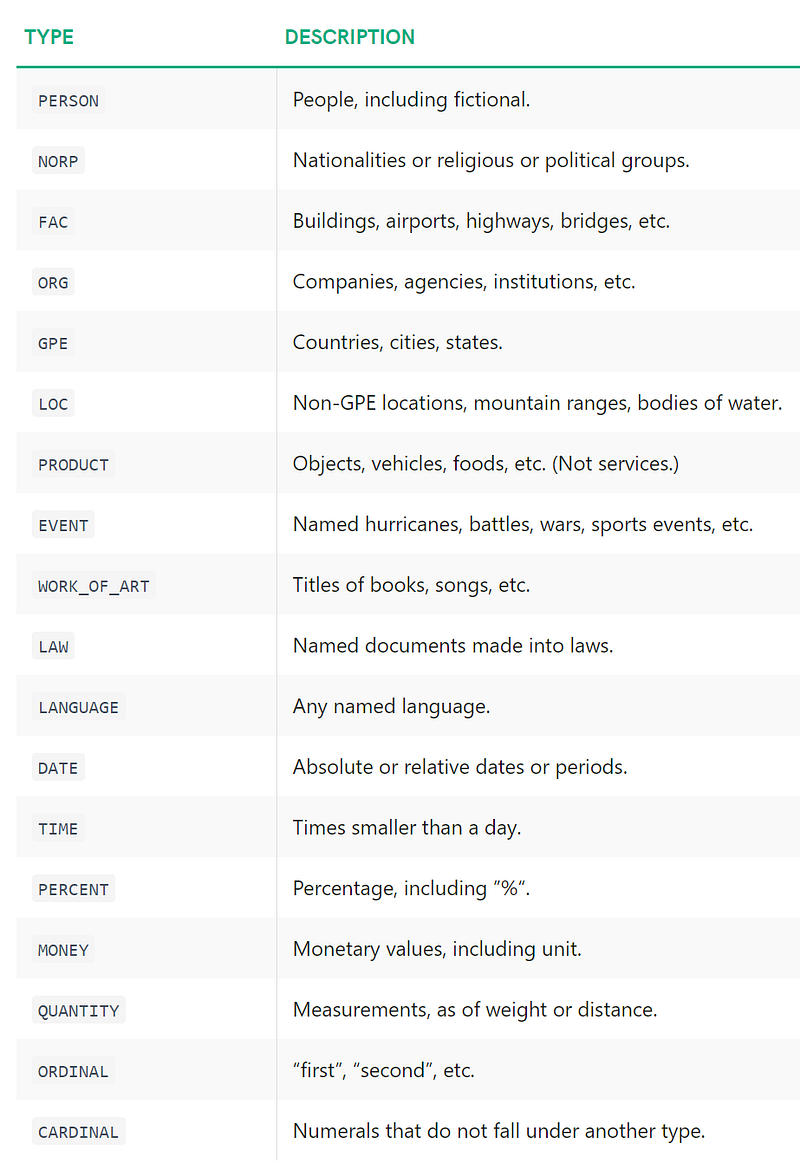
NER (Named-entity recognition) is the process to tag named entities mentioned in unstructured text with pre-defined categories such as person names, organizations, locations, time expressions, quantities, etc.

Training a NER model is really time-consuming because it requires a pretty rich dataset. Luckily there is someone who already did this job for us. One of the best open source NER tools is SpaCy. It provides different NLP models that are able to recognize several categories of entities.

I will give an example using the SpaCy model en_core_web_lg (the large model for English trained on web data) on our usual headline (raw text, not preprocessed):

## call model
ner = spacy.load("en_core_web_lg")

## tag text
txt = dtf["text"].iloc[0]
doc = ner(txt)

## display result
spacy.displacy.render(doc, style="ent")

That’s pretty cool, but how can we turn this into a useful feature? This is what I’m going to do:

• run the NER model on every text observation in the dataset, like I did in the previous example.
• For each news headline, I shall put all the recognized entities into a new column (named “tags”) along with the number of times that same entity appears in the text. In the example, would be

{ (‘Will Smith’, ‘PERSON’):1, (‘Diplo’, ‘PERSON’):1, (‘Nicky Jam’, ‘PERSON’):1, (“The 2018 World Cup’s”, ‘EVENT’):1 }

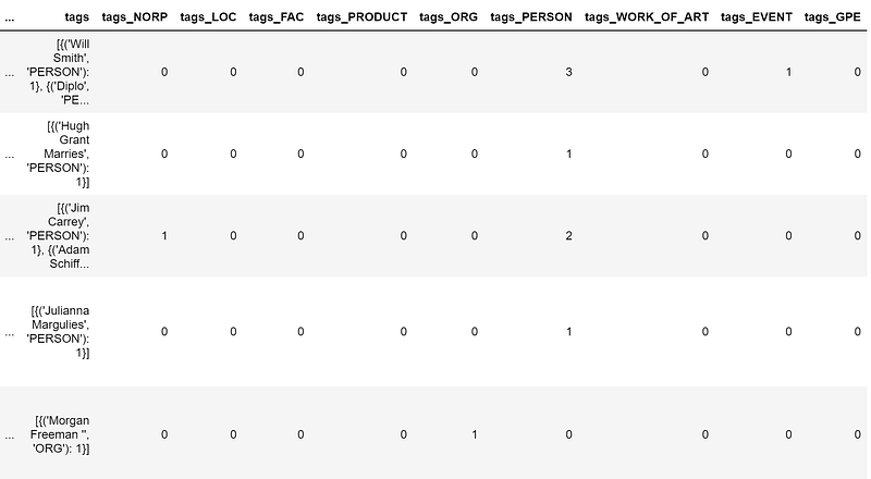
• Then I will create a new column for each tag category (Person, Org, Event, …) and count the number of found entities of each one. In the example above, the features would be

tags_PERSON = 3

tags_EVENT = 1

## tag text and exctract tags into a list
dtf["tags"] = dtf["text"].apply(lambda x: [(tag.text, tag.label_) 
                                for tag in ner(x).ents] )

## utils function to count the element of a list
def utils_lst_count(lst):
    dic_counter = collections.Counter()
    for x in lst:
        dic_counter[x] += 1
    dic_counter = collections.OrderedDict( 
                     sorted(dic_counter.items(), 
                     key=lambda x: x[1], reverse=True))
    lst_count = [ {key:value} for key,value in dic_counter.items() ]
    return lst_count

## count tags
dtf["tags"] = dtf["tags"].apply(lambda x: utils_lst_count(x))

## utils function create new column for each tag category
def utils_ner_features(lst_dics_tuples, tag):
    if len(lst_dics_tuples) > 0:
        tag_type = []
        for dic_tuples in lst_dics_tuples:
            for tuple in dic_tuples:
                type, n = tuple[1], dic_tuples[tuple]
                tag_type = tag_type + [type]*n
                dic_counter = collections.Counter()
                for x in tag_type:
                    dic_counter[x] += 1
        return dic_counter[tag]
    else:
        return 0

## extract features
tags_set = []
for lst in dtf["tags"].tolist():
     for dic in lst:
          for k in dic.keys():
              tags_set.append(k[1])
tags_set = list(set(tags_set))
for feature in tags_set:
     dtf["tags_"+feature] = dtf["tags"].apply(lambda x: 
                             utils_ner_features(x, feature))

## print result
dtf.head()

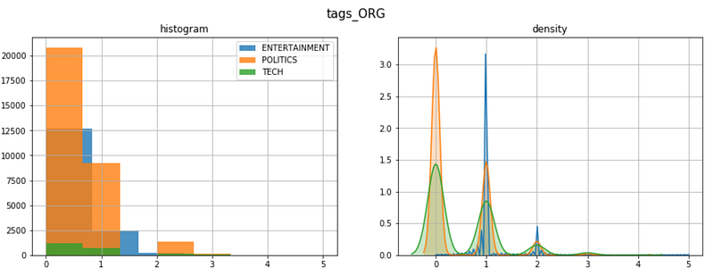
Now we can have a macro view on the tag types distribution. Let’s take the ORG tags (companies and organizations) for example:

In order to go deeper into the analysis, we need to unpack the column “tags” we created in the previous code. Let’s plot the most frequent tags for one of the headline categories:

y = "ENTERTAINMENT"
 
tags_list = dtf[dtf["y"]==y]["tags"].sum()
map_lst = list(map(lambda x: list(x.keys())[0], tags_list))
dtf_tags = pd.DataFrame(map_lst, columns=['tag','type'])
dtf_tags["count"] = 1
dtf_tags = dtf_tags.groupby(['type',  
                'tag']).count().reset_index().sort_values("count", 
                 ascending=False)
fig, ax = plt.subplots()
fig.suptitle("Top frequent tags", fontsize=12)
sns.barplot(x="count", y="tag", hue="type", 
            data=dtf_tags.iloc[:top,:], dodge=False, ax=ax)
ax.grid(axis="x")
plt.show()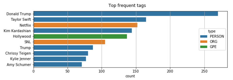

Moving forward with another useful application of NER: do you remember when we removed stop words losing the word “Will” from the name of “Will Smith”? An interesting solution to that problem would be replacing “Will Smith” with “Will_Smith”, so that it won’t be affected by stop words removal. Since going through all the texts in the dataset to change names would be impossible, let’s use SpaCy for that. As we know, SpaCy can recognize a person name, therefore we can use it for name detection and then modify the string.

## predict wit NER
txt = dtf["text"].iloc[0]
entities = ner(txt).ents

## tag text
tagged_txt = txt
for tag in entities:
    tagged_txt = re.sub(tag.text, "_".join(tag.text.split()), 
                        tagged_txt) 

## show result
print(tagged_txt)

Word Frequency

So far we’ve seen how to do feature engineering by analyzing and processing the whole text. Now we are going to look at the importance of single words by computing the n-grams frequency. An n-gram is a contiguous sequence of n items from a given sample of text. When the n-gram has the size of 1 is referred to as a unigram (size of 2 is a bigram).

For example, the phrase “I like this article” can be decomposed in:

• 4 unigrams: “I”, “like”, “this”, “article”
• 3 bigrams: “I like”, “like this”, “this article”

I will show how to calculate unigrams and bigrams frequency taking the sample of Politics news.

y = "POLITICS"
corpus = dtf[dtf["y"]==y]["text_clean"]

lst_tokens = nltk.tokenize.word_tokenize(corpus.str.cat(sep=" "))
fig, ax = plt.subplots(nrows=1, ncols=2)
fig.suptitle("Most frequent words", fontsize=15)
    
## unigrams
dic_words_freq = nltk.FreqDist(lst_tokens)
dtf_uni = pd.DataFrame(dic_words_freq.most_common(), 
                       columns=["Word","Freq"])
dtf_uni.set_index("Word").iloc[:top,:].sort_values(by="Freq").plot(
                  kind="barh", title="Unigrams", ax=ax[0], 
                  legend=False).grid(axis='x')
ax[0].set(ylabel=None)
    
## bigrams
dic_words_freq = nltk.FreqDist(nltk.ngrams(lst_tokens, 2))
dtf_bi = pd.DataFrame(dic_words_freq.most_common(), 
                      columns=["Word","Freq"])
dtf_bi["Word"] = dtf_bi["Word"].apply(lambda x: " ".join(
                   string for string in x) )
dtf_bi.set_index("Word").iloc[:top,:].sort_values(by="Freq").plot(
                  kind="barh", title="Bigrams", ax=ax[1],
                  legend=False).grid(axis='x')
ax[1].set(ylabel=None)
plt.show()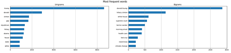

If there are n-grams that appear only in one category (i.e “Republican” in Politics news), those can become new features. A more laborious approach would be to vectorize the whole corpus and use all the words as features (Bag of Words approach).

Now I’m going to show you how to add word frequency as a feature in your dataframe. We just need the CountVectorizer from Scikit-learn, one of the most popular libraries for machine learning in Python. A vectorizer converts a collection of text documents to a matrix of token counts. I shall give an example using 3 n-grams: “box office” (frequent in Entertainment), “republican” (frequent in Politics), “apple” (frequent in Tech).

lst_words = ["box office", "republican", "apple"]

## count
lst_grams = [len(word.split(" ")) for word in lst_words]
vectorizer = feature_extraction.text.CountVectorizer(
                 vocabulary=lst_words, 
                 ngram_range=(min(lst_grams),max(lst_grams)))

dtf_X = pd.DataFrame(vectorizer.fit_transform(dtf["text_clean"]).todense(), columns=lst_words)

## add the new features as columns
dtf = pd.concat([dtf, dtf_X.set_index(dtf.index)], axis=1)
dtf.head()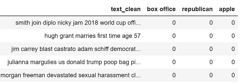

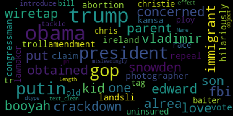
A nice way to visualize the same information is with a word cloud where the frequency of each tag is shown with font size and color.

wc = wordcloud.WordCloud(background_color='black', max_words=100, 
                         max_font_size=35)
wc = wc.generate(str(corpus))
fig = plt.figure(num=1)
plt.axis('off')
plt.imshow(wc, cmap=None)
plt.show()

Word Vectors

Recently, the NLP field has developed new linguistic models that rely on a neural network architecture instead of more traditional n-gram models. These new techniques are a set of language modelling and feature learning techniques where words are transformed into vectors of real numbers, hence they are called word embeddings.

Word embedding models map a certain word to a vector by building a probability distribution of what tokens would appear before and after the selected word. These models have quickly become popular because, once you have real numbers instead of strings, you can perform calculations. For example, to find words of the same context, one can simply calculate the vectors distance.

There are several Python libraries that work with this kind of model. SpaCy is one, but since we have already used it, I will talk about another famous package: Gensim. An open-source library for unsupervised topic modeling and natural language processing that uses modern statistical machine learning. Using Gensim, I will load a pre-trained GloVe model. GloVe (Global Vectors) is an unsupervised learning algorithm for obtaining vector representations for words of size 300.

nlp = gensim_api.load("glove-wiki-gigaword-300")

We can use this object to map words to vectors:

word = "love"

nlp[word]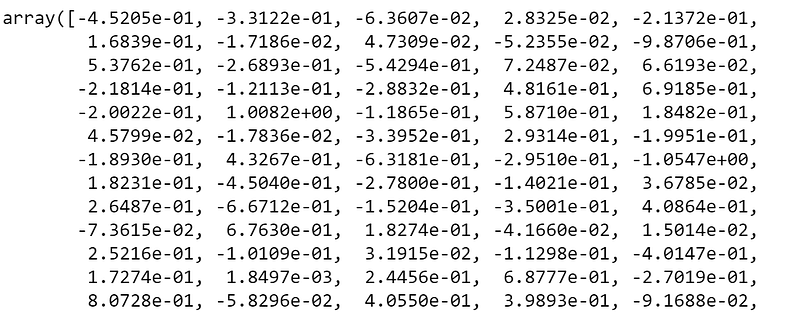

nlp[word].shape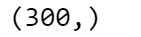

Now let’s see what are the closest word vectors or, to put in another way, the words that mostly appear in similar contexts. In order to plot the vectors in a two-dimensional space, I need to reduce the dimensions from 300 to 2. I am going to do that with t-distributed Stochastic Neighbor Embedding from Scikit-learn. t-SNE is a tool to visualize high-dimensional data that converts similarities between data points to joint probabilities.

## find closest vectors
labels, X, x, y = [], [], [], []
for t in nlp.most_similar(word, topn=20):
    X.append(nlp[t[0]])
    labels.append(t[0])

## reduce dimensions
pca = manifold.TSNE(perplexity=40, n_components=2, init='pca')
new_values = pca.fit_transform(X)
for value in new_values:
    x.append(value[0])
    y.append(value[1])

## plot
fig = plt.figure()
for i in range(len(x)):
    plt.scatter(x[i], y[i], c="black")
    plt.annotate(labels[i], xy=(x[i],y[i]), xytext=(5,2), 
               textcoords='offset points', ha='right', va='bottom')

## add center
plt.scatter(x=0, y=0, c="red")
plt.annotate(word, xy=(0,0), xytext=(5,2), textcoords='offset 
             points', ha='right', va='bottom')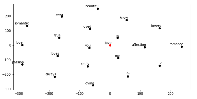

Topic Modeling

The Genism package is specialized in topic modeling. A topic model is a type of statistical model for discovering the abstract “topics” that occur in a collection of documents.

I will show how to extract topics using LDA (Latent Dirichlet Allocation): a generative statistical model that allows sets of observations to be explained by unobserved groups that explain why some parts of the data are similar. Basically, documents are represented as random mixtures over latent topics, where each topic is characterized by a distribution over words.

Let’s see what topics we can extract from Tech news. I need to specify the number of topics the model has to cluster, I am going to try with 3:

y = "TECH"
corpus = dtf[dtf["y"]==y]["text_clean"]

## pre-process corpus
lst_corpus = []
for string in corpus:
    lst_words = string.split()
    lst_grams = [" ".join(lst_words[i:i + 2]) for i in range(0, 
                     len(lst_words), 2)]
    lst_corpus.append(lst_grams)

## map words to an id
id2word = gensim.corpora.Dictionary(lst_corpus)

## create dictionary word:freq
dic_corpus = [id2word.doc2bow(word) for word in lst_corpus] 

## train LDA
lda_model = gensim.models.ldamodel.LdaModel(corpus=dic_corpus, id2word=id2word, num_topics=3, random_state=123, update_every=1, chunksize=100, passes=10, alpha='auto', per_word_topics=True)
   
## output
lst_dics = []
for i in range(0,3):
    lst_tuples = lda_model.get_topic_terms(i)
    for tupla in lst_tuples:
        lst_dics.append({"topic":i, "id":tupla[0], 
                         "word":id2word[tupla[0]], 
                         "weight":tupla[1]})
dtf_topics = pd.DataFrame(lst_dics, 
                         columns=['topic','id','word','weight'])
    
## plot
fig, ax = plt.subplots()
sns.barplot(y="word", x="weight", hue="topic", data=dtf_topics, dodge=False, ax=ax).set_title('Main Topics')
ax.set(ylabel="", xlabel="Word Importance")
plt.show()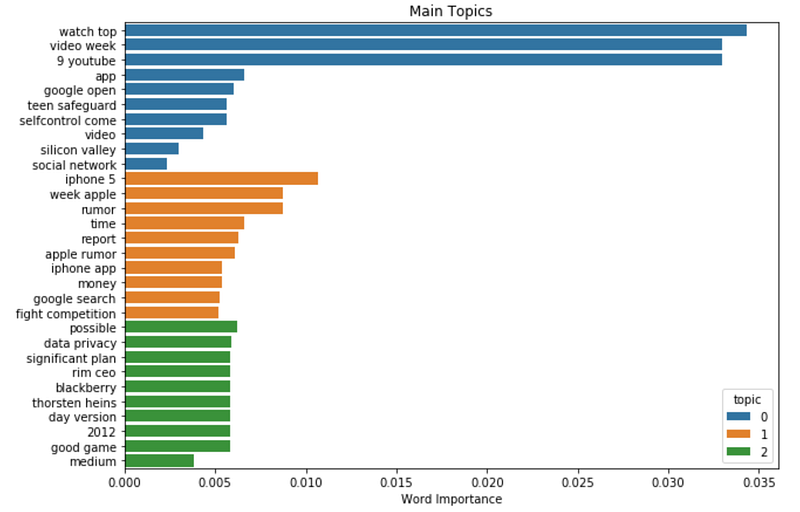

Trying to capture the content of 6 years in only 3 topics may be a bit hard, but as we can see, everything regarding Apple Inc. ended up in the same topic.

Conclusion

This article has been a tutorial to demonstrate how to analyze text data with NLP and extract features for a machine learning model.

I showed how to detect the language the data is in, and how to preprocess and clean text. Then I explained different measures of length, did sentiment analysis with Textblob, and we used SpaCy for named-entity recognition. Finally, I explained the differences between traditional word frequency approaches with Scikit-learn and modern language models using Gensim. Now you know pretty much all the NLP basics to start working with text data.

I hope you enjoyed it! Feel free to contact me for questions and feedback or just to share your interesting projects.

👉 Let’s Connect 👈

This article is part of the series NLP with Python, see also: