Test-Driving Particle Filter: Python Implementation on Stock Prices

Particle filters, also known as Sequential Monte Carlo methods

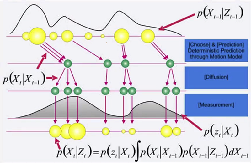
Particle filters are a powerful class of Monte Carlo algorithms used for Bayesian estimation problems, particularly in the context of nonlinear and non-Gaussian state estimation. The particle filter algorithm works by representing the probability distribution of the state using a set of discrete samples called “particles”. Each particle represents a hypothetical state of the system, and the distribution of the particles approximates the true posterior distribution. The algorithm recursively updates the particle weights and positions based on the latest observations, effectively tracking the evolution of the state over time. Particle filters have found widespread application in fields such as robotics, signal processing, finance, and environmental sciences, where they are used for tasks like object tracking, sensor fusion, and time series prediction. Their ability to handle nonlinear and non-Gaussian models, as well as their computational efficiency, make them a valuable tool in a wide range of domains.

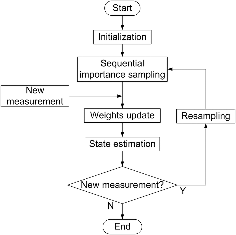
The particle filter algorithm steps are followed closely:

Initialization: Create the particles with a uniform (or normal) distribution.
Prediction: We predict the next state of particles by adding Gaussian (or non-Gaussian) noise.
Update: We update particle weights based on how well they match the actual measurement.
Resampling: We resample particles based on their weights.
Estimation: Computes the estimated state as the mean of the particles.

Let’s install the filterpy library to implement the particle filter to handle non-Gaussian noise environments in robotics.

# https://filterpy.readthedocs.io/en/latest/index.html
pip install filterpy

Imagine you’re tracking a robot’s position in a 2D space, where the robot’s movements and sensor measurements follow non-Gaussian distributions.

import numpy as np
import matplotlib.pyplot as plt
from filterpy.monte_carlo import systematic_resample
from numpy.random import uniform, laplace

# Define the number of particles
num_particles = 1000

# 1. Randomly generate a bunch of particles
particles = uniform(-10, 10, (num_particles, 2))

# Define the state transition function (robot movement) using Laplace distribution
def predict(particles):
    movement_noise = laplace(0, 1, particles.shape)  # Non-Gaussian noise
    return particles + movement_noise

# Define the measurement function (sensor reading)
def measure_distance(particles, target):
    distances = np.linalg.norm(particles - target, axis=1)
    measurement_noise = laplace(0, 1, size=distances.shape)  # Non-Gaussian noise
    return distances + measurement_noise

# Define the likelihood function (importance weight)
def update(particles, weights, target, measured_distance):
    predicted_distances = np.linalg.norm(particles - target, axis=1)
    weights *= np.exp(-0.5 * (predicted_distances - measured_distance)**2)
    weights += 1.e-300  # avoid round-off to zero
    weights /= np.sum(weights)  # normalize
    return weights

# Set the target position (hidden state)
target = np.array([2, 3])

# Initialize weights
weights = np.ones(num_particles) / num_particles

# Store estimated states
estimated_states = []

# Simulate the particle filter over multiple steps
steps = 1000
for _ in range(steps):
    # 2. Predict next state of the particles
    particles = predict(particles)
    
    # 3. Update the weighting of the particles based on the measurement
    measured_distance = measure_distance(particles, target)
    weights = update(particles, weights, target, measured_distance)
    
    # 4. Resample
    indices = systematic_resample(weights)
    particles = particles[indices]
    weights.fill(1.0 / num_particles)
    
    # 5. Compute estimate
    estimated_state = np.mean(particles, axis=0)
    estimated_states.append(estimated_state)
    #print(f"Estimated state: {estimated_state}")

# Convert estimated states to a NumPy array for plotting
estimated_states = np.array(estimated_states)

# Plot the final particles and the target position
plt.figure(figsize=(10, 8))
plt.scatter(particles[:, 0], particles[:, 1], alpha=0.5, label='Particles')
plt.scatter(target[0], target[1], color='red', label='Target')
plt.plot(estimated_states[:, 0], estimated_states[:, 1], color='black', label='Estimated States', linestyle='--')
plt.title(f'Particle Filter with Estimated States over {steps} steps')
plt.xlabel('X position')
plt.ylabel('Y position')
plt.legend()
plt.show()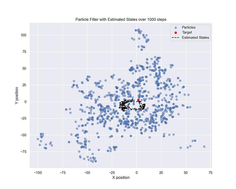

The library provides four types of resampling:

# https://filterpy.readthedocs.io/en/latest/monte_carlo/resampling.html
from filterpy.monte_carlo import systematic_resample 
from filterpy.monte_carlo import residual_resample 
from filterpy.monte_carlo import stratified_resample 
from filterpy.monte_carlo import multinomial_resample

The resampling algorithm significantly affects the performance of the filter. For example, if we resample particles by picking them at random, we would end up choosing many particles with very low weights. This would result in a poor representation of the problem’s probability distribution.

So, while those “resample function” itself doesn’t encompass the entire sequential Monte Carlo sampling process, it is a crucial component of particle filters, which are a type of sequential Monte Carlo method. The function is specifically used in the resampling stage of the particle filter algorithm to help maintain a diverse and representative set of particles throughout the estimation process.

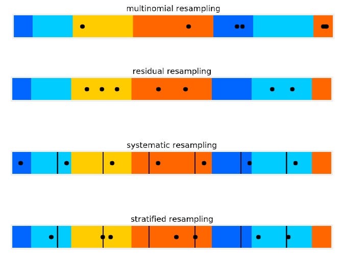
The performance of the multinomial resampling is quite bad. There is a very large weight that was not sampled at all. The largest weight only got one resample, yet the smallest weight was sample was sampled twice.

The residual resampling algorithm does excellently at what it tries to do: ensure all the largest weights are resampled multiple times. It doesn’t evenly distribute the samples across the particles — many reasonably large weights are not resampled at all.

Systematic sampling does an excellent job of ensuring we sample from all parts of the particle space while ensuring larger weights are proportionality resampled more often.

Stratified resampling is not quite as uniform as systematic resampling, but it is a bit better at ensuring the higher weights get resampled more. [3]

Now, let’s implement a particle filter to forecast the closing price of “AAPL” stock.

It’s quite common in financial modeling to use a Gaussian state model with a non-Gaussian measurement model to capture the heavy-tailed nature of returns. In my model, I use Student’s t-distribution as the non-Gaussian measurement model, since the daily return of the “AAPL” closing price exhibits a Student’s t-distribution.

The code will perform a grid search for the following parameters: number of particles, process noise standard deviation, measurement noise standard deviation, and degrees of freedom. It will aim to yield the best R² score. Next, the data will be split into training (80%) and testing (20%) sets. The best parameters found from the grid search will then be used to evaluate the model using multiple metrics on both sets of data.

import yfinance as yf
import numpy as np
import matplotlib.pyplot as plt
from scipy.stats import t as students_t
from filterpy.monte_carlo import systematic_resample, stratified_resample
from sklearn.metrics import r2_score, mean_absolute_error, mean_squared_error
from sklearn.model_selection import train_test_split
import pandas as pd
from itertools import product
import time  
start_time = time.time()  

# Fetch AAPL stock data
data = yf.download("AAPL", start="2020-01-01", end="2024-10-01")
stock_prices = data['Close'].values

def particle_filter(measurements, num_particles, process_std, measurement_std, degrees_of_freedom):
    estimates = []
    
    # 1. Randomly generate initial particles
    particles = np.random.normal(measurements[0], process_std, num_particles)
    
    for measurement in measurements:
        # 2. Predict next state of the particles (State equation / transition model)
        particles = predict_particles(particles, process_std)
        
        # 3. Update the weighting of the particles based on the measurement (Measurement equation / observation model)
        weights = update_weights(particles, measurement, degrees_of_freedom, measurement_std)
        
        # 4. Resample
        particles = resample_particles(particles, weights)
        
        # 5. Compute Estimate
        estimate = compute_estimate(particles)
        estimates.append(estimate)
    
    return estimates

def predict_particles(particles, process_std):
    """State equation / transition model"""
    return particles + np.random.normal(0, process_std, len(particles))

def update_weights(particles, measurement, degrees_of_freedom, process_std):
    """Measurement equation / observation model"""
    weights = students_t.pdf(measurement, df=degrees_of_freedom, loc=particles, scale=process_std)
    weights += 1.e-300  # Avoid divide by zero
    return weights / np.sum(weights)

def resample_particles(particles, weights):
    indices = systematic_resample(weights)
    return particles[indices]

def compute_estimate(particles):
    return np.mean(particles)

# Grid search parameters
num_particles_range = [5000, 7000, 10000, 13000]
process_std_range = [2.0, 5.0, 7.0, 10.0]
measurement_std_range = [1.0, 2.0, 5.0]
degrees_of_freedom_range = [5, 10, 15, 20, 25, 30]

best_r2 = -np.inf
best_params = None

# Perform grid search
for num_particles, process_std, measurement_std, degrees_of_freedom in product(num_particles_range, process_std_range, measurement_std_range, degrees_of_freedom_range):
    estimates = particle_filter(stock_prices, num_particles, process_std, measurement_std, degrees_of_freedom)
    r2 = r2_score(stock_prices, estimates)
    
    if r2 > best_r2:
        best_r2 = r2
        best_params = (num_particles, process_std, measurement_std, degrees_of_freedom)
    
    #print(f"Particles: {num_particles}, Process_Std: {process_std}, Measurement_Std: {measurement_std}, DoF: {degrees_of_freedom}, R2: {r2:.4f}")

print(f"\nBest parameters: Particles: {best_params[0]}, Process_Std: {best_params[1]}, measurement_Std: {best_params[2]}, DoF: {best_params[3]}")

print("\n")
end_time = time.time()  
execution_time = end_time - start_time  
hours, remainder = divmod(execution_time, 3600)  
minutes, seconds = divmod(remainder, 60)   
print(f"Execution time for grid search: {int(hours)} hours, {int(minutes)} minutes, {int(seconds)} seconds")

#=================================================================================================================
#
#
# Split data into training and testing sets
train_prices, test_prices = train_test_split(stock_prices, test_size=0.2, shuffle=False)

# Run particle filter with best parameters on both sets
train_estimates = particle_filter(train_prices, best_params[0], best_params[1], best_params[2], best_params[3])
test_estimates = particle_filter(test_prices, best_params[0], best_params[1], best_params[2], best_params[3])

def calculate_metrics(actual, predicted):
    mae = mean_absolute_error(actual, predicted)
    mse = mean_squared_error(actual, predicted)
    rmse = np.sqrt(mse)
    mape = np.mean(np.abs((actual - predicted) / actual)) * 100
    r2 = r2_score(actual, predicted)
    return {"MAE": mae, "MSE": mse, "RMSE": rmse, "MAPE": mape, "R2": r2}

# Calculate metrics for both sets
train_metrics = calculate_metrics(train_prices, train_estimates)
test_metrics = calculate_metrics(test_prices, test_estimates)

# Print metrics
print("\nTraining Set Metrics:")
for metric, value in train_metrics.items():
    print(f"{metric}: {value:.4f}")

print("\nTesting Set Metrics:")
for metric, value in test_metrics.items():
    print(f"{metric}: {value:.4f}")

# Plotting
plt.figure(figsize=(12, 6))
plt.plot(data.index[:len(train_prices)], train_prices, label='Train Actual', color='blue')
plt.plot(data.index[:len(train_prices)], train_estimates, label='Train Estimate', color='red')
plt.plot(data.index[len(train_prices):], test_prices, label='Test Actual', color='green')
plt.plot(data.index[len(train_prices):], test_estimates, label='Test Estimate', color='orange')
plt.title('AAPL Stock Price: Actual vs Particle Filter Estimate')
plt.xlabel('Date')
plt.ylabel('Stock Price (USD)')
plt.legend()
plt.grid(True)
plt.show()

I was shocked by the results.

Image from https://www.quotes.pics/quote/8228

Best parameters: Particles: 13000, Process_Std: 10.0, measurement_Std: 1.0, DoF: 30


Execution time for grid search: 0 hours, 34 minutes, 33 seconds

Training Set Metrics:
MAE: 0.0247
MSE: 0.0010
RMSE: 0.0321
MAPE: 0.0191
R2: 1.0000

Testing Set Metrics:
MAE: 0.0270
MSE: 0.0013
RMSE: 0.0354
MAPE: 0.0139
R2: 1.0000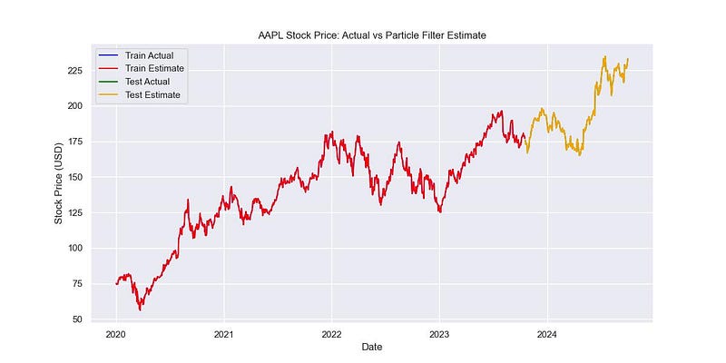

Note that while optimizing for R-squared can improve the fit of your model, it doesn’t necessarily guarantee better forecasting performance. You might want to consider using cross-validation or out-of-sample testing to evaluate the model’s predictive power. (I skipped it)

Disclaimer: The information presented herein is provided solely for informational purposes and should not be construed as financial or investment advice. Any investment decisions or actions taken based on this information are made at your own discretion and risk. Stock prices and investment values are subject to fluctuation due to various market factors and conditions. I strongly recommend consulting with a qualified financial professional for personalized guidance tailored to your individual financial situation and objectives before making any investment decisions.

Thank you for reading

Reference: [1] Particle Filters by Emma Benjaminson [2] GNSS multipath estimation and mitigation based on particle filter [3] Kalman and Bayesian Filters in Python, Roger R Labbe Jr, GitHub (2020);