Technical Pattern Recognition for Trading in Python

Back-testing some Exotic Technical Patterns and evaluating their Performance

Note from Towards Data Science’s editors: While we allow independent authors to publish articles in accordance with our rules and guidelines, we do not endorse each author’s contribution. You should not rely on an author’s works without seeking professional advice. See our Reader Terms for details.

I have just published a new book after the success of New Technical Indicators in Python. It features a more complete description and addition of complex trading strategies with a Github page dedicated to the continuously updated code. If you feel that this interests you, feel free to visit the below link, or if you prefer to buy the PDF version, you could contact me on Linkedin.

The Book of Trading Strategies

Amazon.com: The Book of Trading Strategies (9798532885707): Kaabar, Sofien: Books

www.amazon.com

Pattern recognition is the search and identification of recurring patterns with approximately similar outcomes. This means that when we manage to find a pattern, we have an expected outcome that we want to see and act on through our trading. For example, a head and shoulders pattern is a classic technical pattern that signals an imminent trend reversal. The literature differs on the predictive ability of this famous configuration. In this article, we will discuss some exotic objective patterns. I say objective because they have clear rules unlike the classic patterns such as the head and shoulders and the double top/bottom. We will discuss three related patterns created by Tom Demark:

TD Differential.
TD Reverse-Differential.
TD Anti-Differential.

For more on other Technical trading patterns, feel free to check the below article that presents the Waldo configurations and back-tests some of them:

Where’s Waldo?

Tom Demark, the renowned famous technical analyst has created many successful indicators and patterns. Among his many…

medium.com

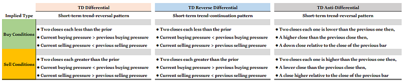
The TD Differential group has been created (or found?) in order to find short-term reversals or continuations. They are supposed to help confirm our biases by giving us an extra conviction factor. For example, let us say that you expect a rise on the USDCAD pair over the next few weeks. You have your justifications for the trade, and you find some patterns on the higher time frame that seem to confirm what you are thinking. This will definitely make you more comfortable taking the trade. Below is a summary table of the conditions for the three different patterns to be triggered.

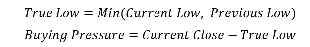
Summary of conditions for the three price patterns. (Image by Author)

Before we start presenting the patterns individually, we need to understand the concept of buying and selling pressure from the perception of the Differentials group. To calculate the Buying Pressure, we use the below formulas:

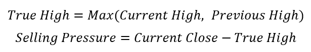
To calculate the Selling Pressure, we use the below formulas:

Now, we will take them on one by one by first showing a real example, then coding a function in python that searches for them, and finally we will create the strategy that trades based on the patterns. It is worth noting that we will be back-testing the very short-term horizon of M5 bars (From November 2019) with a bid/ask spread of 0.1 pip per trade (thus, a 0.2 cost per round).

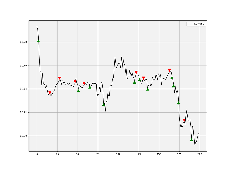
TD Differential Pattern

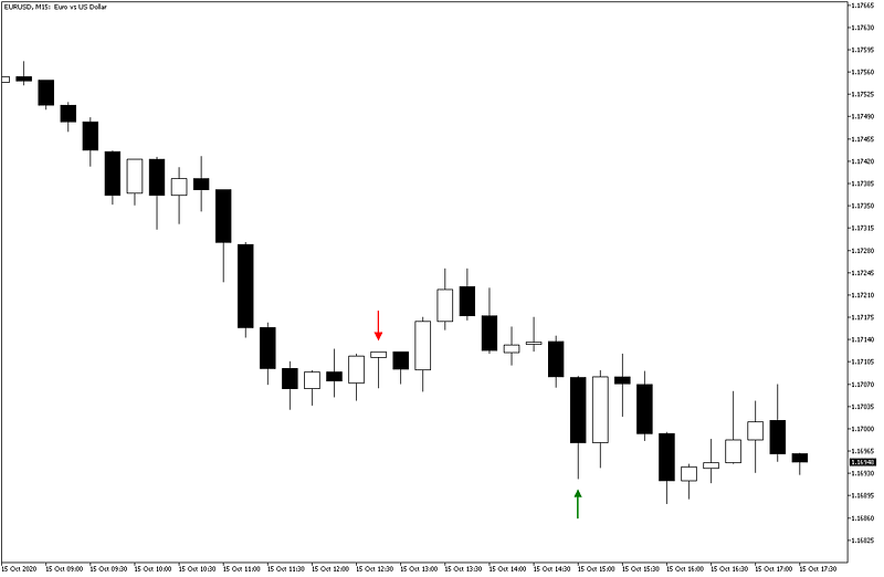
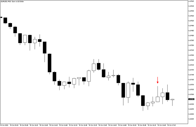
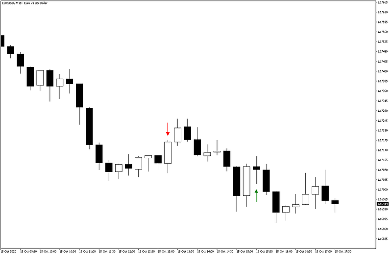
This pattern seeks to find short-term trend reversals; therefore, it can be seen as a predictor of small corrections and consolidations. Below is an example on a candlestick chart of the TD Differential pattern.

Example of the Pattern. Notice the Short-term tendancy of the Reaction. (Image by Author)

If we want to code the conditions in Python, we may have a function similar to the below:

Buy (Go long) trigger:

Two closes each less than the prior.
Current buying pressure > previous buying pressure.
Current selling pressure < previous selling pressure.

Sell (Go short) trigger:

Two closes each greater than the prior.
Current buying pressure < previous buying pressure.
Current selling pressure > previous selling pressure.

def TD_differential(Data, true_low, true_high, buy, sell):
    for i in range(len(Data)):
        
        # True low
        Data[i, true_low] = min(Data[i, 2], Data[i - 1, 3])
        Data[i, true_low] = Data[i, 3] - Data[i, true_low]
            
        # True high  
        Data[i, true_high] = max(Data[i, 1], Data[i - 1, 3])
        Data[i, true_high] = Data[i, 3] - Data[i, true_high]
        
        # TD Differential
        if Data[i, 3] < Data[i - 1, 3] and Data[i - 1, 3] < Data[i - 2, 3] and \
           Data[i, true_low] > Data[i - 1, true_low] and Data[i, true_high] < Data[i - 1, true_high]: 
               Data[i, buy] = 1

if Data[i, 3] > Data[i - 1, 3] and Data[i - 1, 3] > Data[i - 2, 3] and \
           Data[i, true_low] < Data[i - 1, true_low] and Data[i, true_high] > Data[i - 1, true_high]: 
               Data[i, sell] = -1

Now, let us back-test this strategy all while respecting a risk management system that uses the ATR to place objective stop and profit orders. I have found that by using a stop of 4x the ATR and a target of 1x the ATR, the algorithm is optimized for the profit it generates (be that positive or negative). It is clear that this is a clear violation of the basic risk-reward ratio rule, however, remember that this is a systematic strategy that seeks to maximize the hit ratio on the expense of the risk-reward ratio.

Reminder: The risk-reward ratio (or reward-risk ratio) measures on average how much reward do you expect for every risk you are willing to take. For example, you want to buy a stock at $100, you have a target at $110, and you place your stop-loss order at $95. What is your risk reward ratio? Clearly, you are risking $5 to gain $10 and thus 10/5 = 2.0. Your risk reward ratio is therefore 2. It is generally recommended to always have a ratio that is higher than 1.0 with 2.0 as being optimal. In this case, if you trade equal quantities (size) and risking half of what you expect to earn, you will only need a hit ratio of 33.33% to breakeven. A good risk-reward ratio will take the stress out of pursuing a high hit ratio.

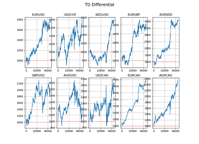
Example of a Signal Chart on the EURUSD — TD Differential Pattern. (Image by Author)

Equity Curves of the TD Differential Strategy on 10 Major Currency Pairs. (Image by Author)

It looks like it works well on AUDCAD and EURCAD with some intermediate periods where it underperforms. Also, the general tendency of the equity curves is upwards with the exception of AUDUSD, GBPUSD, and USDCAD. For a strategy based on only one pattern, it does show some potential if we add other elements. If we take a look at an honorable mention, the performance metrics of the AUDCAD were not bad, topping at 69.72% hit ratio and an expectancy of $0.44 per trade.

If you are also interested by more technical indicators and using Python to create strategies, then my best-selling book on Technical Indicators may interest you:

New Technical Indicators in Python

Amazon.com: New Technical Indicators in Python: 9798711128861: Kaabar, Mr Sofien: Books

www.amazon.com

TD Reverse-Differential Pattern

This pattern seeks to find short-term trend continuations; therefore, it can be seen as a predictor of when the trend is strong enough to continue. It is useful because as we know it, the trend is our friend, and by adding another friend to the group, we may have more chance to make a profitable strategy. Let us check the conditions and how to code it:

Example of the Pattern. (Image by Author)

Buy (Go long) trigger:

Two closes each less than the prior.
Current buying pressure < previous buying pressure.
Current selling pressure > previous selling pressure

Sell (Go short) trigger:

Two closes each greater than the prior.
Current buying pressure > previous buying pressure.
Current selling pressure < previous selling pressure

def TD_reverse_differential(Data, true_low, true_high, buy, sell):
    for i in range(len(Data)):
        
        # True low
        Data[i, true_low] = min(Data[i, 2], Data[i - 1, 3])
        Data[i, true_low] = Data[i, 3] - Data[i, true_low]
            
        # True high  
        Data[i, true_high] = max(Data[i, 1], Data[i - 1, 3])
        Data[i, true_high] = Data[i, 3] - Data[i, true_high]
        
        # TD Differential
        if Data[i, 3] < Data[i - 1, 3] and Data[i - 1, 3] < Data[i - 2, 3] and \
           Data[i, true_low] < Data[i - 1, true_low] and Data[i, true_high] > Data[i - 1, true_high]: 
               Data[i, buy] = 1

if Data[i, 3] > Data[i - 1, 3] and Data[i - 1, 3] > Data[i - 2, 3] and \
           Data[i, true_low] > Data[i - 1, true_low] and Data[i, true_high] < Data[i - 1, true_high]: 
               Data[i, sell] = -1

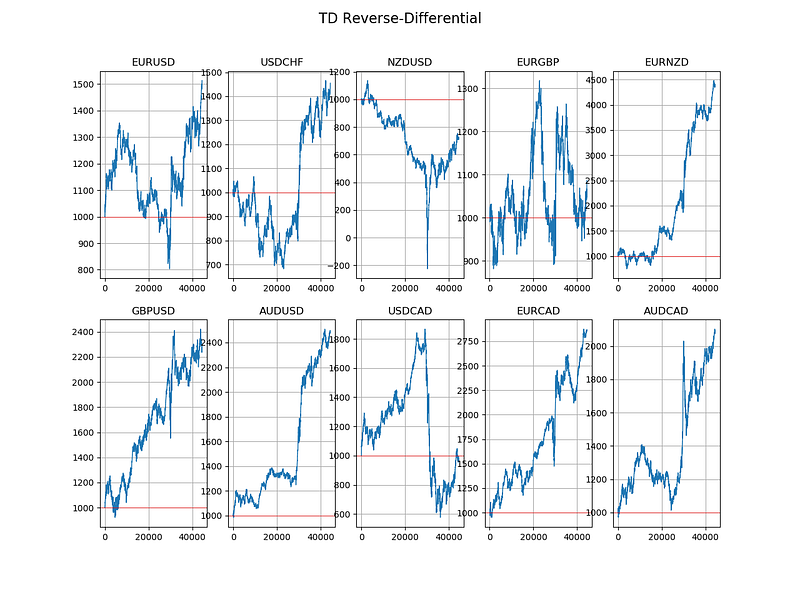
Example of a Signal Chart on the EURUSD — TD Reverse-Differential Pattern. (Image by Author)

Equity Curves of the TD Reverse-Differential Strategy on 10 Major Currency Pairs. (Image by Author)

It looks like it works well on GBPUSD and EURNZD with some intermediate periods where it underperforms. The general tendency of the equity curves is less impressive than with the first pattern. If we take a look at some honorable mentions, the performance metrics of the GBPUSD were not too bad either, topping at 67.28% hit ratio and an expectancy of $0.34 per trade.

TD Anti-Differential Pattern

This pattern also seeks to find short-term trend reversals, therefore, it can be seen as a predictor of small corrections and consolidations. It is similar to the TD Differential pattern. The following are the conditions followed by the Python function.

Buy (Go long) trigger:

Two closes each one is lower than the previous one then,
A higher close than the previous close then,
A lower close relative to the close of the previous bar.

Sell (Go short) trigger:

Two closes each one is higher than the previous one then,
A lower close than the previous close then,
A close higher relative to the close of the previous bar.

def TD_anti_differential(Data, true_low, true_high, buy, sell):
    for i in range(len(Data)):
        
        if Data[i, 3] < Data[i - 1, 3] and Data[i - 1, 3] > Data[i - 2, 3] and \
           Data[i - 2, 3] < Data[i - 3, 3] and Data[i - 3, 3] < Data[i - 4, 3]: 
               Data[i, buy] = 1

if Data[i, 3] > Data[i - 1, 3] and Data[i - 1, 3] < Data[i - 2, 3] and \
           Data[i - 2, 3] > Data[i - 3, 3] and Data[i - 3, 3] > Data[i - 4, 3]: 
               Data[i, sell] = -1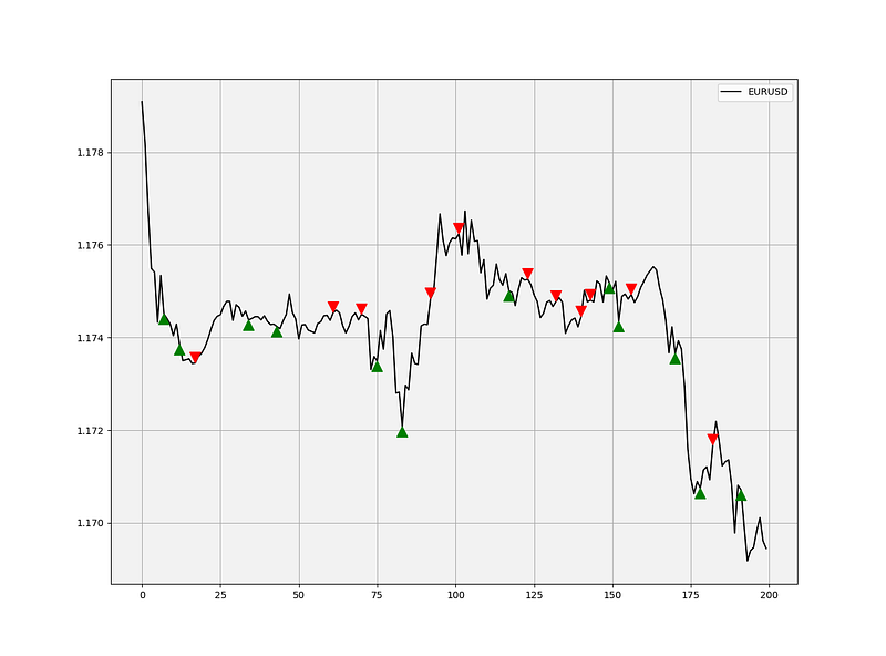

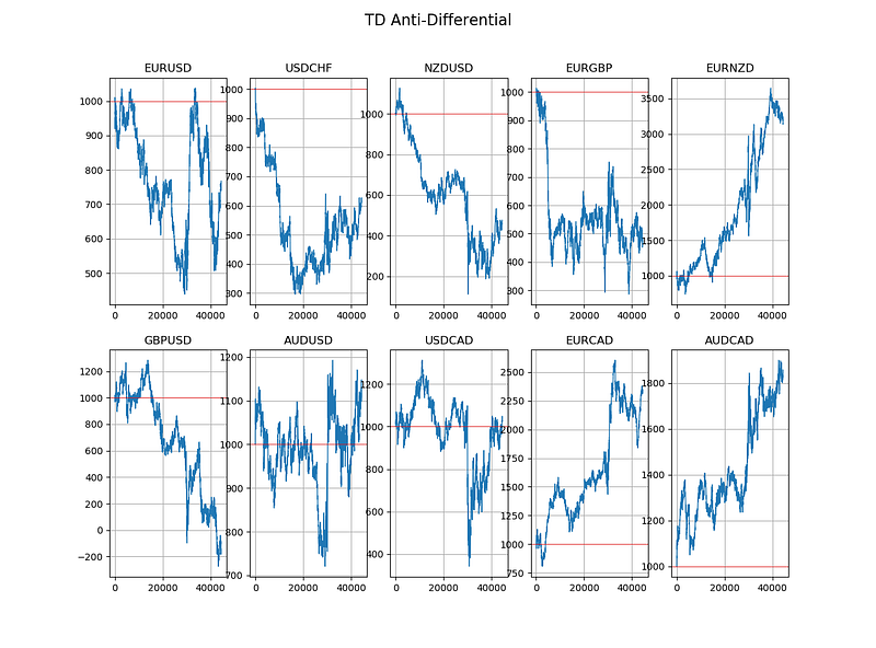
Example of a Signal Chart on the EURUSD — TD Anti-Differential Pattern. (Image by Author)

Equity Curves of the TD Anti-Differential Strategy on 10 Major Currency Pairs. (Image by Author)

It looks much less impressive than the previous two strategies. The general tendency of the equity curves is mixed. If we take a look at some honorable mentions, the performance metrics of the EURNZD were not too bad either, topping at 64.45% hit ratio and an expectancy of $0.38 per trade.

Remember, the reason we have such a high hit ratio is due to the bad risk-reward ratio we have imposed in the beginning of the back-tests. With a target at 1x ATR and a stop at 4x ATR, the hit ratio needs to be high enough to compensate for the larger losses.

Conclusion

I am always fascinated by patterns as I believe that our world contains some predictable outcomes even though it is extremely difficult to extract signals from noise, but all we can do to face the future is to be prepared, and what is preparing really about? It is anticipating (forecasting) the probable scenarios so that we are ready when they arrive. In The Book of Back-tests, I discuss more patterns relating to candlesticks which demystifies some mainstream knowledge about candlestick patterns.

I always advise you to do the proper back-tests and understand any risks relating to trading. For example, the above results are not very indicative as the spread we have used is very competitive and may be considered hard to constantly obtain in the retail trading world. However, with institutional bid/ask spreads, it may be possible to lower the costs such as that a systematic medium-frequency strategy starts being profitable.