Talk data to me — Modeling of Singapore Grand Prix 2018

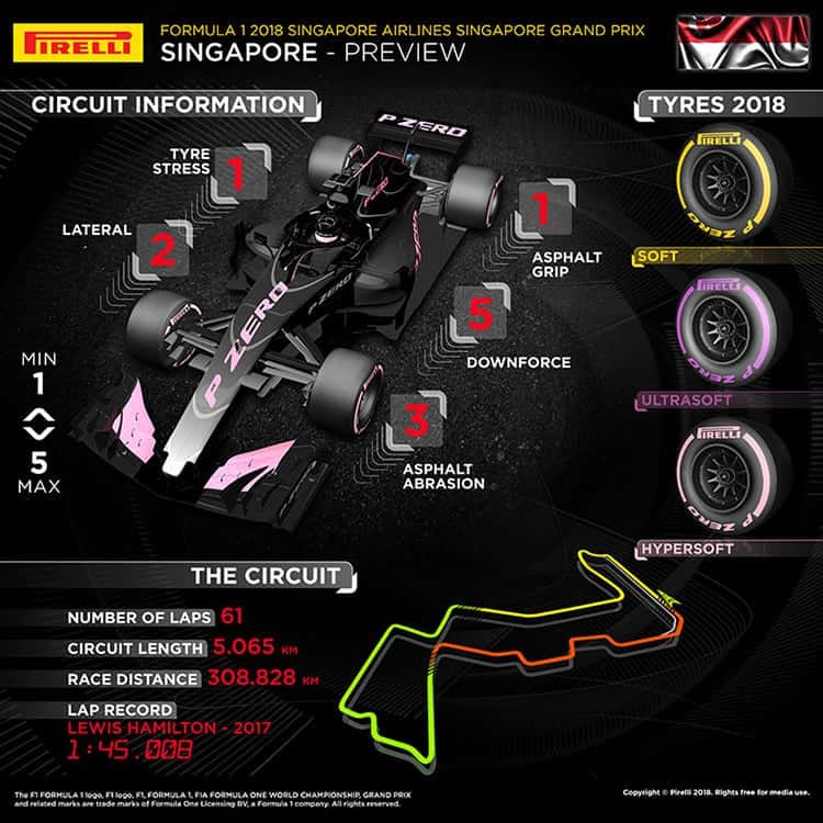
The Marina Bay Street Circuit, also known as the “Singapore Street Circuit” is a street circuit around Singapore’s Marina Bay, which has been hosting the Singapore Grand Prix every year since 2008. Due to Singapore’s yearly high temperatures, its humidity and the uneven nature of the street track and the heavy braking zones, the Singapore Circuit represents a physical challenge for both the drivers and cars, and it is probably the most demanding race on the F1 calendar. Moreover, it is the longest race of Formula One Grand Prix season, taking up to two hours to complete.

Background

Having read the 2018 world cup predictions reports by various banks, I decided to embark on my own journey to do my own data analysis and predictive modeling of the upcoming F1 race in Singapore. This short article will cover the challenges faced, lessons learnt and of course the results of the models and predictions. It will be split it into 5 sections — data mining, data processing and exploration, feature engineering, model building and the final results. This side project was mainly done after office hours, and thus I did not have much time for it. The plan was to come up with a detailed report by start of qualifications, but this is what I have currently, and plan to improve it even after the Singapore Grand Prix is over.

Data Mining

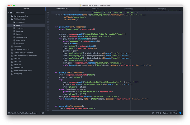
Mainly, I found two amazing free-for-all sites which gave me the necessary data I needed to work with, the Ergast F1 data repository, and of course the official Formula1 website. Both data sources have essentially the same data, but having more than one source of data is excellent as I was able to cross validate and ensure data accuracy, which is very important in any data science project. However, I was initially despondent when I saw the data on the official site, which I was planning to rely heavily on. It had no good API end points, or downloadable links which I can easily dump the data locally. Therefore, I spent some time coding out a spider to crawl the official F1 site automatically, format it nicely for me, and dump it in a CSV file which I can work on. It was a pain in the arse to code it out, as there were many caveats I had to consider for the site. Each website is different, and thus I needed to go through the front end code to really pry it open and extract the data from within. Looking back, building a custom scraper for it was too time-consuming, and not worth the effort if I am not coming back for data often, which is in this case as F1 races are only annually. Web scrapers are most worth the effort if the data is updated on a high frequency, and you want to have the freshest data mined periodically. I can go on to talk about the many challenges I faced even in this data mining process, but it would too long. I plan to attach/upload the spider so you can take a look at the source code and run it yourself.

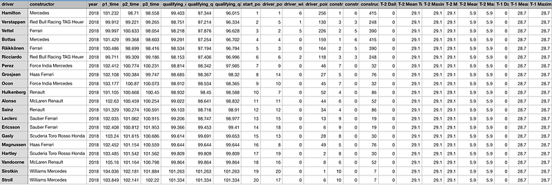
To prevent data leakage and achieve model viability, I only used features that will be available to public before the final race, such as practice timings, qualification timings, current standing, constructor/driver stats and weather data. Final features that was considered are:

'driver', 'constructor', 'year', 'p1_time', 'p2_time', 'p3_time', 'qualifying_q1', 'qualifying_q2', 'qualifying_q3', 'start_position', 'driver_pos', 'driver_wins', 'driver_points', 'constructor_pos', 'constructor_wins', 'constructor_points',
'T-2 Daily Rainfall Total (mm)', 'T-2 Mean Temperature (°C)',
'T-2 Maximum Temperature (°C)', 'T-2 Minimum Temperature (°C)',
'T-2 Mean Wind Speed (km/h)', 'T-2 Max Wind Speed (km/h)',
'T-1 Daily Rainfall Total (mm)', 'T-1 Mean Temperature (°C)',
'T-1 Maximum Temperature (°C)', 'T-1 Minimum Temperature (°C)',
'T-1 Mean Wind Speed (km/h)', 'T-1 Max Wind Speed (km/h)',
'T-0 Daily Rainfall Total (mm)', 'T-0 Mean Temperature (°C)',
'T-0 Maximum Temperature (°C)', 'T-0 Minimum Temperature (°C)',
'T-0 Mean Wind Speed (km/h)', 'T-0 Max Wind Speed (km/h)',
'T-0 Humidity', 'factor_q1', 'factor_q2', 'factor_q3'

Exploratory Data Analysis

After gathering the data, I deciding on the following data points to be included in the machine learning model. My final data set consists of 3 sections. First section is primary data set such as qualification and practice timing,

'final_time', 'p1_time','p2_time', 'p3_time', 'qualifying_q1', 'qualifying_q2', 'qualifying_q3',

2nd part is weather data such as weather numbers for all 3days,

‘T-0 Humidity’,
 ‘T-0 Max Wind Speed (km/h)’, ‘T-0 Maximum Temperature (°C)’,
 ‘T-0 Mean Temperature (°C)’, ‘T-0 Mean Wind Speed (km/h)’,
 ‘T-0 Minimum Temperature (°C)’, ‘T-1 Daily Rainfall Total (mm)’,
 ‘T-1 Max Wind Speed (km/h)’, ‘T-1 Maximum Temperature (°C)’,
 ‘T-1 Mean Temperature (°C)’, ‘T-1 Mean Wind Speed (km/h)’,
 ‘T-1 Minimum Temperature (°C)’, ‘T-2 Daily Rainfall Total (mm)’,
 ‘T-2 Max Wind Speed (km/h)’, ‘T-2 Maximum Temperature (°C)’,
 ‘T-2 Mean Temperature (°C)’, ‘T-2 Mean Wind Speed (km/h)’,
 ‘T-2 Minimum Temperature (°C)’

and lastly the third part will be proxy psychological data, that includes the drivers and teams current standing data. I hope this would capture confidence level, and current aptitude to a certain degree.

'constructor_points', 'constructor_pos',
       'constructor_wins', 'driver_points', 'driver_pos', 'driver_wins',
       'factor_q1', 'factor_q2', 'factor_q3', 'start_position'

These are the free data I have found within my limited time. Since I have only 10 years of Singapore Grand Prix data, and each race has ~20 drivers each, altogether I would have ~200 rows, which is extremely extremely small for a data science project. Machine learning models work well with large data sets, which goes minimally to around 100k+ rows/observation. Unless I scope it in another manner, I have to make do with 200 rows. I supplemented it with getting as many features as possible, and using simple machine learning algorithms such as decision trees K-nearest neighbours which handles small datasets well. If I had the time, I would try Gaussian Mixture Model — GMM or a Kernel Density Estimation — KDE model to fit to the data, and maybe create more sample points according to the distribution to supplement the dataset.

After much data mangling and processing, (I can attest that 80% of a data scientist’s time is spend collecting and cleaning data to be fed into a model), we have to do some exploratory data analysis, to get a feel of the data, and thus having a clearer idea of what we are working with.

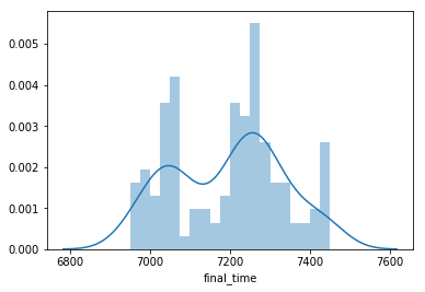
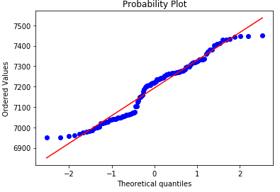
First we plot out the target viable, which is final_timing in the regressions case. We can see that the final timing for the drivers are not normally distributed, bimodal in fact, which in this case traditional statistical modeling may not perform as well as machine learning algorithms. We need to use a model that has as little prior assumptions as possible, remember Oscam’s razor principle from philosophy.

In brevity, I did a few charts to get a ‘feel’ of the data, and this are a few interesting looking ones that tell alot about the data. Can you find some interesting points and tell a story from them?

g = sns.PairGrid(df, vars=['final_time', 'p1_time', 'p2_time', 'p3_time','qualifying_q1','qualifying_q2','qualifying_q3'],
                hue='year')
g.map(plt.scatter, alpha=0.8)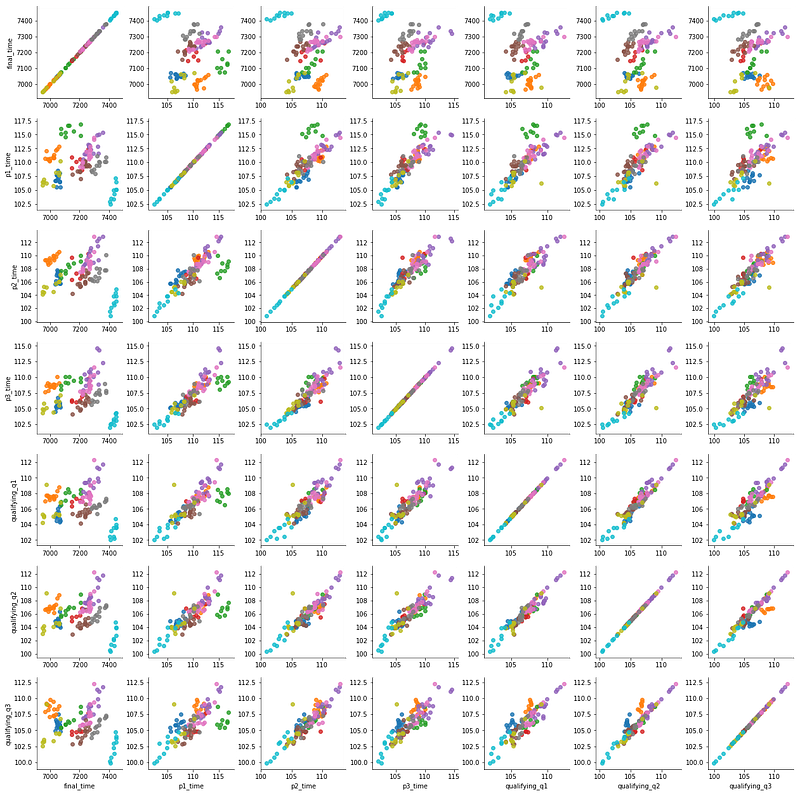

We can see from above that there a few outliers, see the first row light blue dots. They are data from 2017, which shows that they perform really well in the practice and qualification races, and did really badly in the final race, which does not make sense. After some investigation, I have yet to understand the cause, if any of you have any ideas do let me know. I was considering whether to remove the outliers, as I have to weigh in the benefits of removing, against the cost of an even smaller dataset. I decided to leave it in, as there were sufficient variance in the other independent variables to prove sufficient hidden pattern use case.

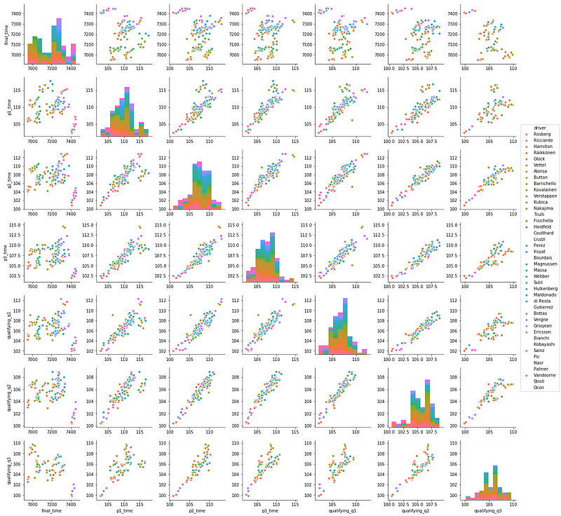
The next diagram shows the pair wise features according to the drivers, as color hues.

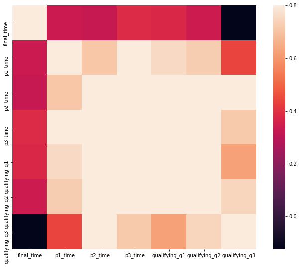
Below is the correlation matrix that calculate the covariance among features. A covariance matrix C should be positive (semi-)definite and hence satisfies |Cij|2 ≤ Cii Cjj for all indices i, j. Consequently, the absolute values of the entries of the corresponding correlation matrix do not exceed 1. It seems like practice 3 timings as the highest correlation with our target variable.

Feature Engineering

The main consideration here for feature engineering is the values for missing qualification 1, qualification 2, and qualification 3 timings. The way qualification stages in Formula One work is that everyone will be racing for the fastest lap in each stage, and the slowest few will be cut off from the next stage. Q3 will then be left with 10 of the 20 drivers and they will be racing for pole position. Hence, there will be missing values for Q2 and Q3 timings. The issue now is how to deal with them. I considered both imputing 0, and the mean value of their qualification timings. I chose to stick with the latter since it gives better CV results. I then engineered dummy variables to indicate if they have qualified for each round so as to differentiate the good timings from the mean imputed ones that may indicate a false sense of caliber.

Reliability of CV in our special small dataset case

(Reserved for later)

Model building

Here comes the fun part. My total dataset will be split into 3 parts, training set, validation set and testing set. 80% will be kept and trained on, to help with hyper-parameter of the top few machine learning model that performs well on this current dataset. 20% will then be kept for the testing phase which will help me decide on the final model to use. You can imagine how much smaller my dataset will become after setting aside data. Woes of a small dataset. I thus expect the whole modelling process to either overfit the little data, or generalize too much with low variance without capturing sufficient information pattern, if I use too much regularization. Below are some snippets of code for model building, with their scores and performance metrics.

The best peforming ML algorithms for the regression problem are tree-based algos, such as xgboost, and gradient boosted machines. This is expected given the small dataset we have, gradient boosting seems to work much better, however, overfitting is very possible too.

Best algorithms for classification seem to be generative parametric models such as Gaussian Naive Bayes and plain old logistic regression due to the small dataset. Personally, the biggest reason for me to use classification algos is that the output will be probablities, and thus give us a level of confidence in our predictions. Simple models are preferred in this case over complex ones like neural networks or support vector machines, given the small data set.

Results

Today is Sunday, 4:15pm SGT, and we have the necessary data to feed into our models. Weather data is not the most updated given the punctuality of data upload from third party website, or rather, the lack of it. I acknowledge that it is impossible to predict the future with absolute certainty and accuracy, and the modeling is done with the absence of black swan events such as crashes and mechanical failures of cars. Therefore take all predictions not as absolutes, but as one of the many probable outcomes that may happen.

I cycled through a few machine learning algorithms and cross-validated them using default hyper-parameters. Gaussian Naive Bayes was found to perform the best for the classification use case, as a simple model that handles small data set well, by avoiding overfitting. All it needs is just enough data to understand the probabilistic relationship of each attribute in isolation with the output variable. If we remember, the Naive Bayes model implements the conditional independence assumption of variables, which states:

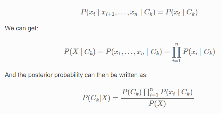
Here, we can see the conditional independence assumption allows us to decompose the joint probability into the product of its individual conditional probability. Given this assumption, interactions between attributes are ignored in the NB model, and therefore less data is required than other algorithms, such as logistic regression.

The output probabilities are

array([[  9.86946284e-01,   7.28337599e-10,   1.30537153e-02,
          1.72345949e-18],
       [  4.15098562e-03,   8.11719387e-01,   1.84089277e-01,
          4.03497370e-05],
       [  8.84896982e-01,   5.53190939e-06,   1.15097486e-01,
          7.33192226e-13],
       [  5.72129249e-01,   2.95752186e-01,   1.32118095e-01,
          4.70342962e-07],
       [  6.24334562e-01,   5.23328111e-02,   3.23332557e-01,
          6.95170040e-08],
       [  1.05800315e-02,   8.30211885e-01,   1.59133366e-01,
          7.47173402e-05],
       [  3.02710585e-15,   9.65307033e-05,   1.26336566e-12,
          9.99903469e-01],
       [  1.03314187e-12,   3.21719528e-03,   2.51658972e-09,
          9.96782802e-01],
       [  1.13571219e-17,   5.74930398e-07,   7.64280974e-20,
          9.99999425e-01],
       [  9.95552765e-13,   1.74366411e-03,   5.68711596e-05,
          9.98199465e-01],
       [  4.25041679e-17,   5.34682515e-06,   2.97058108e-15,
          9.99994653e-01],
       [  9.74673511e-19,   2.70610655e-05,   8.30072791e-07,
          9.99972109e-01],
       [  1.53744062e-38,   2.81243243e-13,   1.89234750e-18,
          1.00000000e+00],
       [  6.43947469e-50,   5.80549592e-16,   1.04393210e-21,
          1.00000000e+00],
       [  2.55984480e-37,   1.02107891e-16,   3.50864801e-32,
          1.00000000e+00],
       [  1.28104715e-22,   8.33318547e-12,   1.05361704e-19,
          1.00000000e+00],
       [  7.11591872e-52,   2.52345170e-21,   2.18606142e-38,
          1.00000000e+00],
       [  3.38169675e-42,   7.28193346e-20,   1.43783647e-41,
          1.00000000e+00],
       [  7.84282427e-64,   3.52150114e-28,   1.94456020e-50,
          1.00000000e+00],
       [  2.63062818e-64,   2.00881810e-28,   2.62750991e-45,
          1.00000000e+00]])

Using relative probabilities, the prediction from Gaussian Naive Bayes model is 1st Hamilton[98.7%], 2nd (Ricciardo[83%]/Verstappen[81.2%]), 3rd Vettel[88.5%] model is quite confident of first, however not so as compared to Hamilton’s 98.7%, therefore relegates to second which model is confident it will NOT happen with an absolute 0%. Thus third is chosen]. One thing to note is that the interpretation of probabilities here is very tricky as there are different ways to scope the percentages. I have yet to incorporate the intuition of having only exclusive positions as the model sometimes assigns more than 1 first/second placing (eg. 1 1 2 3 3).Thus for relative % we look at where the model is very confident of a placing (>80% confidence level) and scope it from there. If a confident prediction is overshadowed by another even higher prediction %, it will be relegated to the next position in line. Therefore, relative probability positioning looks at other driver’s probabilities too before assigning final position.

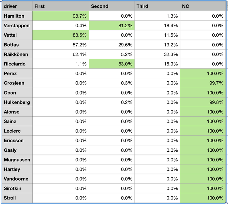
Looking at the highest probabilities for each category, we have 1st Hamilton, 2nd Ricciardo, 3rd Raikkonen if we regard objective probabilities. However, the disadvantage of using this method, is that the model’s confidence of a certain placing is being overlooked in certain cases. (Case in point_: Vettel)

Results from an optimised Extreme Gradient Boosted(xgboost) regressor are as follows. I prefer the simpler faster Naive Bayes model as it works really well with our small dataset, as compared to xgboost which tends to overfit smaller datasets.

array([ 7163.32324219,  7195.625     ,  7166.68261719,  7181.12939453,
        7177.8671875 ,  7209.40185547,  7228.80029297,  7244.18994141,
        7241.67675781,  7235.10058594,  7243.78613281,  7244.70361328,
        7251.99169922,  7250.84033203,  7245.22216797,  7245.1875    ,
        7257.49560547,  7261.64306641,  7258.93945312,  7257.22021484], dtype=float32)

which results to the prediction: 1st Hamilton, 2nd Vettel, 3rd Räikkönen, Bottas, Verstappen, Ricciardo, Perez, Hulkenberg, Ocon, Alonso, Grosjean, Sainz, Magnussen, Gasly, Ericsson, Leclerc, Stroll, Hartley, Sirotkin, Vandoorne of finishing in that order.

This project was really fun to do, and I wished I had more time to build on it, with additional data points, feature engineering, or dimensionality reduction techniques to remove correlated features that may confuse our NB model.