|NEURAL NETWORKS|TABULAR LEARNING| DEEP LEARNING|

Tabula Rasa: How to save your network from the category drama

Neural networks do not like categories but you have techniques to save your favorite model

Tree-based models are still the preferred choice of data scientists for medium-sized tabular data. In the previous article we addressed, what are the challenges of tabular data, why decision trees seem to work best, why we would like to use neural networks instead, and what criteria are needed for a neural network for tabular data.

Instead, in this article we will discuss what strategies have been tried and what deep learning models have been designed for dealing with categorical data.

This article is divided into different sections, for each section we will answer these questions:

• An introduction to tree-based models. What is a decision tree? what are the advantages and the limitations? how do we solve their limits?
• What are tree ensembles? Why they are useful? Which type of ensembles are?
• How you can deal with categorical variables with neural networks? Which techniques can you use? From simple to more sophisticated techniques

Check the list of references at the end of the article, I provide also some suggestions to deepen the topics.

The tree dominion

Tabular data are everywhere. Despite their complexity, they are among the first data to be created and analyzed. That is why there is extensive literature on tabular data and the machine learning models that have been created and used.

Everything is based on a basic unit or the building block of so many models: the decision tree.

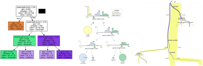
A decision tree is a predictive model expressed as a recursive partition of the covariates space to subspaces that constitute a basis for prediction. The decision tree consists of nodes. (source)

In simple words starting from a root node, the dataset is divided (split) according to the best feature, using a criterion to evaluate which is the best split. The dataset is split until no more partitions can be made.

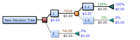
One of the advantages of decision trees is that they can be linearized into decision rules, which makes them easy to interpret (and you can even render them visually)

Decision trees have been successful because they have a number of advantages:

• They are computationally efficient, scale well with data, and at the same time have good performance.
• They are capable of handling different types of data (nominal, numeric, and textual), they are nonparametric (do not hold assumptions about space distribution) and there are versions that can handle missing data.
• They are self-explainable can be used for various tasks, and also usually work well with initial parameters.

However, decision trees have a number of disadvantages:

• the “divide and conquer” strategy only works well if there are some highly relevant attributes.
• it is defined as “myopic” because only one level at a time is considered to overlook a combination of features.
• it is unstable because if a split near the root changes (perhaps due to noise in the dataset) the whole substructure changes.
• it is fragmented if several attributes are tested and if there are many features the cost O(logn) can get expensive.

Unity is strength

Individually, we are one drop. Together, we are an ocean. — Ryunosuke Satoro

To solve these shortcomings, it was decided to combine multiple trees into a single model (ensemble). the idea is to take advantage of the so-called wisdom of the crowd (consulting different opinions before deciding). The idea of a decision forest began in the 1970s but was later realized in the early 1990s.

Why do decision forests work so well?

The theoretical basis of decision forests starts from Condorcet’s jury theorem as early as 1785. According to this theorem, imagining a jury having to vote on a binary problem (where each juror has p > 0.5 of being correct) the probability that the majority of voters are correct approaches 1 as the number of jurors increases. That is, though, if the jurors are independent.

The main advantages of an ensemble are:

• When there is little data, the learning algorithm must choose one model among several that perform equally well. A decision forest simply allows you to choose them all and assign a weight to the predictions.
• The hypothesis space sometimes does not contain a tree that perfectly fits the data. Combining several trees allows for a better fit by extending the hypothesis space.
• A decision tree can end up in local minima, an ensemble decreases this risk
• the tradeoff between variance and bias errors. A small decision tree has high bias but low variance error, increasing the depth of the tree increases the variance bias (and decreases the bias). ensemble techniques decrease both the bias and the variance parts of the error.

A forest of ensemble algorithms

The success of the ensemble has led to the design of a great many algorithms. Although an extended discussion of the topic is not the focus of this article, in brief, it can be said that the strategies for merging the outputs of the various weak learners (single decision tree) are mainly two:

• Weighting methods. Each individual tree output is associated with a weight. This strategy in its simplest form is majority voting (e.g., the final class of the model is equal to the majority of the votes of the ensemble trees), but there are also strategies where the accuracy of each tree is taken into account for its vote. or where voting is combined.
• Meta-learning methods. In this case, we have a process with at least two stages, where the various individual trees are trained (first stage) and then a meta-model is trained. The role of the meta-model is to generate the final output as a function of the outputs of the individual trees.

Of note is the bagging technique, where each individual learner is trained on only a subset of the examples (or even a subset of the features). This strategy is for example used in a random forest, in which the tree chooses the best from a random set of features.

Adaptive boosting is another popular alternative, in which case the algorithm gives more weight to instances that are misclassified. Trees are trained sequentially, and subsequent trees focus on the most difficult examples.

Gradient-boosted decision Trees are similar to AdaBoost, except that gradient descent is used to minimize error in sequential models. XGBoost takes this concept to the extreme by exploiting parallelization, tree pruning, and so on.

The name xgboost, though, actually refers to the engineering goal to push the limit of computations resources for boosted tree algorithms. Which is the reason why many people use xgboost. — Tianqi Chen, creator of the library, source

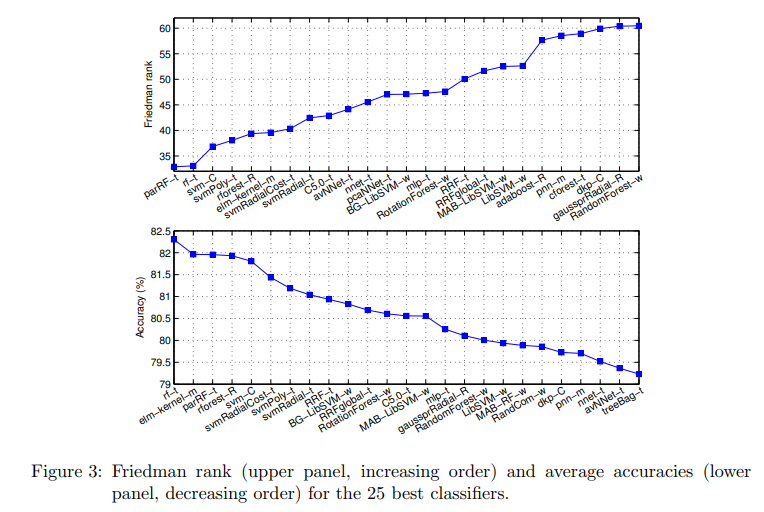
Different studies have shown that random forest has been shown to be superior to other models and alternatives. Subsequently, in various benchmarks, XGBoost showed better performance and lower training time.

Another popular alternative was presented in 2017: Catboost. This algorithm was designed with the purpose of improving the treatment of categorical variables. To date, it is one of the most widely used tree-based algorithms on Kaggle. One of the most interesting new features is the fact that the model uses oblivious trees (which are very efficient on CPU) and overfit less.

LightGBM is 6 times faster than XGBoost (so more efficient with big data) although it is more sensitive to overfitting with small datasets. LightGBM grows tree leaf-wise while other algorithms grow level-wise, which is linked to lower error trees faster than level-wise.

Another interesting model is Explainable Boosting Machine whose focus is explainability: “Explainable Boosting Machine (EBM) is a tree-based, cyclic gradient boosting Generalized Additive Model with automatic interaction detection.” For the authors, the model has competitive performances with black-box models (Random Forest and Boosted Trees) though it is much more interpretable.

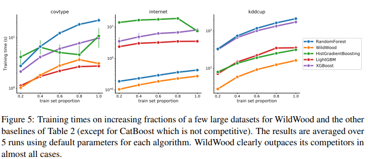
Despite, today’s boosting-based algorithms being preferred over random forestry the search is still active. XGBoost and other freedoms are under active development, and today XGBoost is almost as fast as LightGBM. In addition, a random forest-based model, WildWood, has recently come out and claims to be superior to XGBoost (both in accuracy and training time).

Transform tabular data for neural network

The universe is transformation: life is opinion. — Marcus Aurelius

As we have mentioned, deep learning models have been enormously successful on homogeneous data (images, text, audio). For heterogeneous data, tree-based models have often been used. Interest in deep learning models resurged when e-commerce applications began to be successful. Indeed, the latter produces huge amounts of tabular data with particularly sparse matrices. So different potential algorithms were tested.

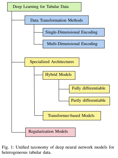
Recently, a unified taxonomy of models has been proposed that divides tabular deep learning approaches into three categories: data transformation methods, specialized architectures, and regularization models.

We leverage this classification to explore the various models that have been proposed.

Transform your dataset

Traditional approaches have sought to transform the dataset so that it is as suitable as possible for neural networks. As has been noted for images and text, preprocessing is minimal while for tabular data the choice of preprocessing can have dramatic effects.

One of the issues that have been most faced is how to deal with categorical variables. This is because a product/user matrix can grow rapidly with the encoding of categorical variables. Second, neural networks accept only numeric input variables so you have to transform the categories into numeric format.

In general, we can define two families of methods:

• Single-Dimensional Encoding
• Multi-Dimensional Encoding.

Single-Dimensional Encoding

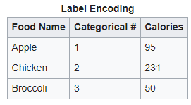
This group is actually composed of two subgroups: deterministic techniques and algorithm techniques. deterministic techniques are preprocessing techniques that are applied before training. Label encoding is the simplest method; each possible label is assigned an integer (for example, {Italy, France} and is mapped to {0,1}). Label encoding inserts an artificial order between variables, during gradient descent the larger label values will contribute more to the weights update.

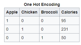
One-hot encoding is another technique in which a categorical variable with a distinct set of labels n, leads to generating a vector v of size n, where it will be 1 for the corresponding label i and 0 for the rest. For example, {Italy, France} is mapped into two columns and an example with the prim label will have a vector [1,0] and instead [0,1] for the second label. Considering that a column is added for each category, in case there are many categories it can lead to a very sparse matrix. Which increases both computation and storage time. On the other hand, it has the advantage that it can be used as a pre-step for embedding and is also running time efficiently.

Two other disadvantages: first, the assumption among categorical features should be independent, but as cardinality (the number of different categories) increases, features begin to interact. Second, since not all categories are equally represented at high cardinality it makes it difficult for the model to learn the rare categories.

Dummy encoding is much similar but instead, we use k-1 dummy variables. For example, for {Italy, France, and Germany} we would have only two columns. For Italy, we would have a vector [1,0], for France instead [0,1] and Germany [0,0]. The real difference is that for one of the categories we use a vector containing only 0. Effect Encoding is a very similar technique (also called Deviation Encoding or Sum Encoding), where instead of using 0 and 1, we use three different values: 1, 0, and -1.

Binary encoding is another technique in which a categorical variable is encoded using the binary format for the number. Here again, columns are added to divide the various digits, but considering a number n of classes we need log(n) columns. For example for {Italy, France, Germany}, we will have only two columns, and the vectors produced will be: [0,1], [1,0], [1,1].

leave-one-out encoding is a technique that does not generate additional columns. In the column itself, the label is replaced by the average of its frequency (excluding that row at the time of calculation). It has the advantage of compressing into one column, but it can be expensive to compute if you have big data.

Hashing, on the other hand, is a technique in which a hash function is used to convert categorical values into numerical values. The hash function can also be very complex, but generally simple functions are used. Hashing is chosen when the number of labels is so large that one-hot encoding becomes too expensive. On the other hand, one must be sure to maintain the mapping and that there are not too many hash collisions.

Target encoding is a Baysian encoding technique where you replace each category with a blend of the posterior probability of the target.

Multi-Dimensional Encoding

Since word2vec was designed to transform textual information into a vector representation (real numbers) it was thought to test the same approach for categorical variables. The idea is precisely to learn a distributed representation that allows categorical variables to be mapped to numeric vectors. Typically, these are called automatic methods of transforming categorical variables.

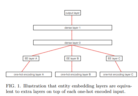
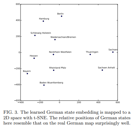
Entity embedding. This is an example of embedding for categorical variables and was used in a 2015 Kaggle competition. The authors successfully showed that by using a simple Keras embedding layer a good result could be achieved. After conducting one-hot coding for categorical variables, they simply fed the embedding layer.

the aim of the competition was to predict Rossman Store Sales in Germany. Interesting, how what is learned from embedding maintains relationships and can then also be leveraged.

VIME is another approach in which one can conduct the encoding of categorical variables in a self or semi-supervised manner. the idea is that VIME trains an encoder that transforms both categorical and numeric variables into a new homogenous representation.

In general, it can be said that the idea of transforming tabular data into a homogenous format has gotten particular attention in recent years because CNNs and transformers are very efficient with images and text. Therefore, there are examples of work proposing to transform tabular data as images. One example is SuperTML, which transforms tabular data into black-and-white images (2D matrices). The first step is to achieve embedding, after which these matrices are simply rearranged to achieve embedding.

A similar method is image generator for tabular data (IGTD). In this case, the authors exploit the fact that CNNs have a bias for spatial dependencies, to do so the authors aim to optimize the distance between pixels as a function of the distance between features in the tabular dataset.

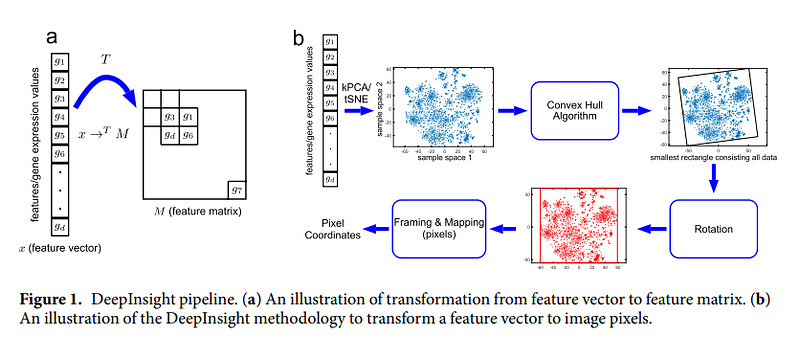
But there are also other approaches such as DeepInsight instead exploit t-sne to generate images from tabular data. REFINED (REpresentation of Features as Images with NEighborhood Dependencies) which instead exploits Bayesian multidimensional scaling to project figures into a 2-D space. Or methods such as OmicsMapNet exploit a priori domain knowledge (in this case feature-specific knowledge) for projection into 2-D space

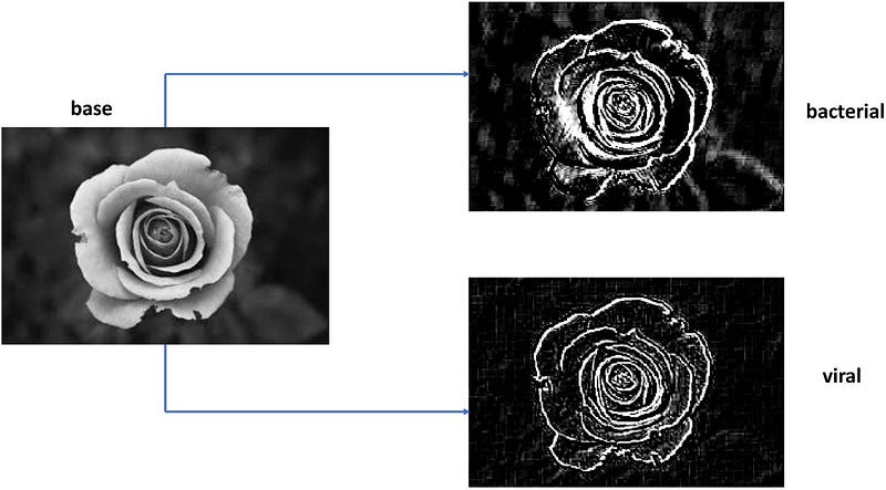
The examples seen above have a limitation, if there are few features that generate few pixels. This can make it difficult for convolutional networks to classify. So in one study, they decided to use transfer learning and adapt it to the case of tabular data. As the authors state, convolutional networks that have been trained on millions of images have higher accuracy than the human eye. These networks have learned an immense number of patterns and it is much more convenient to exploit this knowledge than to re-train it from scratch.

The process is to transform a feature vector (for each example we have a feature vector), rearrange it into a square matrix, and subtract the mean value:

The convolutional kernels used in image processing are typically a square matrix with odd number of rows and columns (e.g., 3 × 3, 5 × 5, 7 × 7 etc). Hence, feature vectors can be directly converted to kernels if the number of features is a square of an odd integer greater than 1 (i.e., number of features must be 9, 25, 49 etc). (source)

In other words rearranged our feature vector into a square matrix (if needed we add padding or remove features with low variance) and normalized. At this point, we take an image and use the matrix obtained earlier as a filter for a convolution.

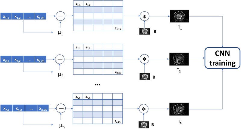
So we get an image for example (and all using one basic image). The authors then used this approach to classify gene expression data from 2,590 blood samples from patients with an infectious disease (bacterial or viral). The result is that the two classes of examples lead to different images after convolution, and the convolutional network has good results

In general, these methods work well when features have strong relationships or you have solid knowledge about the features. In case, however, the features are independent or one cannot characterize the similarity between the features these methods may fail.

Parting thoughts

Tabular data is still one of the most difficult frontiers for machine learning models. While deep learning has outperformed any other model for homogeneous data (images, text, audio, video, graphs) it still has suboptimal performance for tabular data.

As we saw in the previous article, one of the main challenges is that the data is heterogeneous. Tabular data can be composed of both continuous and categorical variables. While it is easy for decision trees to find a split for categorical variables, neural networks have more difficulty in learning an optimal representation of these types of variables. Although decision trees can be used for categorical variables, newer models have found even better solutions to this problem.

In this article, we have seen how it is possible to transform categorical variables so that they can be used as inputs to neural networks. As we have seen over the years, increasingly sophisticated techniques have been developed. These techniques allow us to avoid having to discard categorical variables when we use tabular datasets as inputs to neural networks. At the same time, there is still a long way to go to have an efficient neural network model with tabular data. In the next articles, we will explore other elegant solutions for making neural networks efficient with tabular learning.

What do think? Let me know in the comments

Next article of the series:

If you have found this interesting:

You can look for my other articles, and you can also connect or reach me on LinkedIn.

Here is the link to my GitHub repository, where I am planning to collect code and many resources related to machine learning, artificial intelligence, and more.

or you may be interested in one of my recent articles:

Reference

Here is the list of the principal references I consulted to write this article, only the first name for an article is cited.

1. Rikach, 2016, Decision forest: Twenty years of research, link
2. IBM, Decision Trees, link
3. Zhang, 2021, Dive into Decision Trees and Forests: A Theoretical Demonstration, link
4. Louppe, 2014, Understanding Random Forests: From Theory to Practice, link
5. Delgado, 2014 Do we Need Hundreds of Classifiers to Solve Real World Classification Problems?, link
6. Kaggle, LightGBM Classifier in Python, link
7. Ke, 2017, LightGBM: A Highly Efficient Gradient Boosting Decision Tree, link
8. Prokhorenkova, 2019, CatBoost: unbiased boosting with categorical features, link
9. Lou, 2013, Accurate intelligible models with pairwise interactions, link
10. Gaiffas, 2021, WildWood: a new Random Forest algorithm, link
11. Borisov, 2021, Deep Neural Networks and Tabular Data: A Survey, link
12. Hancock, 2020, Survey on categorical data for neural networks, link
13. Guo, 2016, Entity Embeddings of Categorical Variables, link
14. Dahouda, 2021, A Deep-Learned Embedding Technique for Categorical Features Encoding, link
15. Yoon, 2020, VIME: Extending the Success of Self- and Semi-supervised Learning to Tabular Domain, link
16. Sun, 2019, SuperTML: Two-Dimensional Word Embedding for the Precognition on Structured Tabular Data, link
17. Zhu, 2021, Converting tabular data into images for deep learning with convolutional neural networks, link
18. Sharma, 2019, DeepInsight: A methodology to transform a non-image data to an image for convolution neural network architecture, link
19. Bazgir, 2020, Representation of features as images with neighborhood dependencies for compatibility with convolutional neural networks, link
20. Ma, 2018, OmicsMapNet: Transforming omics data to take advantage of Deep Convolutional Neural Network for discovery, link
21. Avanzi, 2023, Machine Learning with High-Cardinality Categorical Features in Actuarial Applications, link
22. Buturovic, 2020, A novel method for classification of tabular data using convolutional neural networks, link
23. Saupin Guillaume, Transfer learning with XGBoost and PyTorch: Hack Alexnet for MNIST dataset, link
24. Saupin Guillaume, Tuning XGBoost with XGBoost: Writing your own Hyper Parameters Optimization engine, link
25. Saupin Guillaume, XGBoost explained: DIY XGBoost library in less than 200 lines of python, link
26. Saupin Guillaume, How can XGBoost support natively categories?, link