Swin Transformer 🚀: Hierarchical Vision Transformer using Shifted Window — Part I

Microsoft Research, ICML’21 -🏆Marr Prize

This article is the third paper of the “Transformers in Vision” series, which comprises summaries of the recent advanced papers, submitted in the year range of 2020–2022, to top conferences, focusing on transformers in vision.

*NerdFacts-🤓 have additional intricate details, which you can skip and still be able to get a high-level flow of paper!

✅ Background

After the booming entry of Vision Transformer in 2021, the research community became hyperactive for improving classic ViT👁️, because original ViTs were very data-hungry and were trained on in-house google JFT-300M private dataset, which generalized the idea that ViTs can’t be used off the shelf for image classification.

So Facebook AI’s team came up with DeiT ⚗️, which is a data-efficient transformer and was able to out-perform SOTA convolutional networks and ViTs, in terms of accuracy/FLOPs trade-off. DeiT was trained on no external data but just ImageNet21. But it used distillation and depended on a convolution network for knowledge distillation, so was not completely a convolution-free solution.

Both DeiT and ViT, were just tested and designed for Image classification, with the general perception that, if a network architecture performs good for the image classification task, it is expected to do good on others because, “image classification is used as a benchmark for measuring the progress of a technique in the vision domain, any progress here translates to downstream tasks like detection and segmentation”. There is no other work in my knowledge, that used ViT or DeiT as a feature extraction backbone, for tasks other than classification.

Microsoft Research Asia jumped in with SWIN transformer 🚀, with the idea of making VisionTransformer more generic and adaptable for other vision tasks. In all deep learning solutions, we have a deep neural network (like CNN in Computer vision and Transformer in NLP) that is used for extracting features, this network is called backbone. Extracted features are passed into an appropriate head based on the end goal, like classification/detection or sentiment analysis/translation.

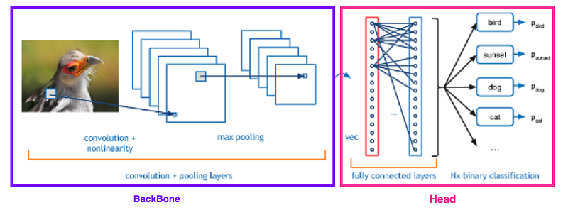
SWIN Transformer 🚀, was presented as a general-purpose backbone for computer vision tasks, that can be used off-the-shelf to perform classification, detection and segmentation, better than SOTA convolutional networks, ViT and DeiT.

[NerdFacts-🤓 : This paper was awarded a highly honorable David Marr Prize at ICML’21 conference, because of its smart design and performance.]

1. Swin Transformer 🚀

Swin Transformer is one of my favorite architectures in Vision. Transformers were originally built for performing machine translation. Speech is temporal data and has no spatial aspect to it, unlike images, Therefore, classic global self-attention-based transformers did pretty well on translation tasks as they were perfect for capturing long-range dependencies.

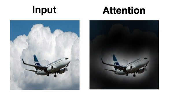
When it comes to images, for classifying an image or detecting a cat in a corner of an image, attending all pixels or patches(image crop) is of no use. This idea can be confirmed from the ablation studies of ViT, as they computed global attention among all patches and found out, just encoder layers were paying attention just to the local region with the object!

Hence for images, one needed to modify not just the network architecture but the attention mechanism inside Transformer’s Encoder block too! — SWIN’s authors morphed global attention to local attention and made a general-purpose Transformer backbone in Computer Vision.

2. SWIN Transformer🚀 Architecture

I’ll try to easily explain the main components of SWIN first and then we’ll put all pieces together to get the final model.

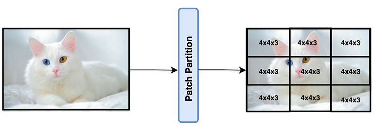
2.1 Patch Partition

An image is passed through a SWIN transformer by dividing it into non-overlapping patches, just like ViT. Each patch is called a token and is of size 4x4x3=48 pixels, where 3 is for the RGB channel and 4 is the height and width of the square patch.

2.2 Patch Merging

Patch merging is an important most crucial layer in SWIN transformer architecture as it induces the inductive bias in SWIN, that was missing from classic ViT and DeIT.

[ NerdFact-🤓: Transformers are permutation invariants, means if you reorder the input and pass it through an encoder you will still get the same output, that is why we add positional encodings, but simple positional encodings are not enough for capturing the spatial correlations in an image, as we saw in ViT, but SWIN is not permutation invariant, you’ll now by the end of the article WHY?]

Patch Merging combines 2x2 windows, and merge them into one new window, downsampling feature map size by 2x and increases depth of each patch by2.

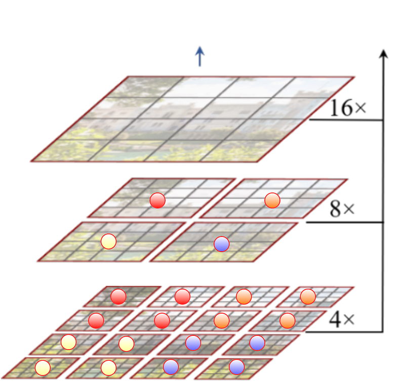
Let’s dive into details! After dividing an image into patches, image patches are grouped into windows, such that each window has MxM patches.

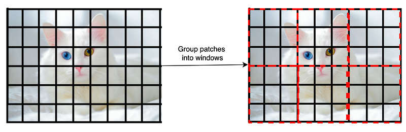
For our cat example image, windowing patches look like this. Here each window has 3x3 patches, so M=3. In the paper, each window has MxM = 7x7 patches. And each patch is 4x4x3=48 pixels.

Now, these windows are grouped and merged together. The authors took 2x2 windows and merged them to make a single window in the next stage. In the below hypothetical example figure from the paper, red dotted windows at 4x level, merged together to make a single window at 8x level. Similarly, all four windows at level 8x, are merged together to make one window at level 16x. Also, note that the number of patches in the new window after merging still remains MxM.

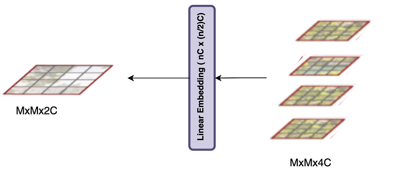
But how do we take 4 windows and merge them to make one window of the same size? Well… we put 4 windows on top of each other so that each patch’s dimension becomes 4C from C, now we pass each patch through a linear layer, which projects the dimension of the output patch to 2C from 4C and we get MxMx2C output merged patch!

2.3 Self Attention in a Window (W-MSA)

SWIN transformer uses Encoder blocks from the original Transformer architecture. Each encoder block is made of a multi-headed self-attention module and a feed-forward network. In a ViT, The multi-headed self-attention uses dot product-based attention for computing attention encodings of each patch, w.r.t all other patches in an input image. So in the figure given below, for ViT, on right, if we want to compute attention for the top-left green patch, we attend to all other tokens, which becomes quadratic in computation!

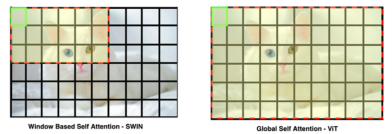
In SWIN, we take a fixed-sized window, such that each window has a fixed number of patches. Our window, in the left figure, has, 3x6 patches, in paper authors, take square windows and each window has MxM patches. Now for computing attention encoding of the top left patch, we just attend to the patches in this window. This approach is a lot more efficient and scalable than attending to all tokens for every token. Authors called this attention, Windowed multi-headed self-attention, W-MSA.

2.4 Self Attention Across “Shifted” Windows (SW-MSA)

If we just rely on window based attention, then the correlations between windows would be missing, and they are important for performing vision tasks, at least that’s what the increasing receptive field of a CNN teaches us!🧐

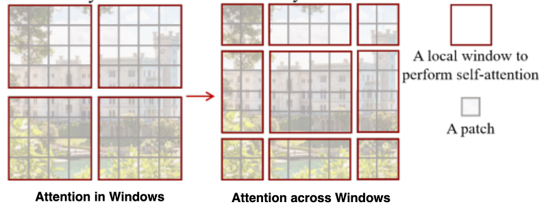
The above figure is an illustrative example used by authors in the paper. Left is the self-attention computed in a window. Each window has 4x4 patches. So, for capturing the attention across windows, the Authors used a smart approach of

1. Taking the output of the W-MSA
2. Shifting all windows by half of their height and width
3. Compute W-MSA in shifted windows

This attention is called SW-MSA, shifted windowed multi-headed self-attention.

In this example image, shifting all 4 windows by 4/2=2 patches down and then 2 patches left, will give you new shifted windows on right. Border windows are not of MxM size in shifted windowed attention, and that’s obvious; to avoid this in CNNs, we pad image to apply a filter on borders. What did the authors of SWIN do to avoid this?

2.4.1 Efficient Computation of Shifted Windows ⚙️

Well… in SWIN authors could have just padded the smaller windows too! but as the number of windows is increasing from h x w to (h+1)x(w+1), [2x3 -> 3x3], it makes the computational complexity grow. “ Reducing inference time is critical because it can later be traded off with accuracy by using larger networks.” (src)

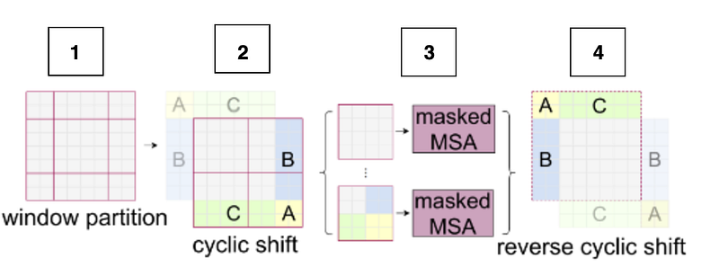
So we want to compute 1. Imagine we take the window given in 2, and shift it down and left by 2x2. then we take patches from A, B, and C and fill them in the empty spaces. Now we take each window in 3, and mask regions as shown in the image, to make sure attention is computed among the desired parts in a window. Finally, in 4, we reverse shift the window and fill the top left part of the new window with patches from the bottom right and repeat! This process allows to compute cross window attention efficiently as the number of windows remains the same as WMSA.

2.5 SWIN Transformer🚀 Block

Now let’s climb up the tree and make a SWIN transformer🚀 block from the W-MSA and SW-MSA we just learned!

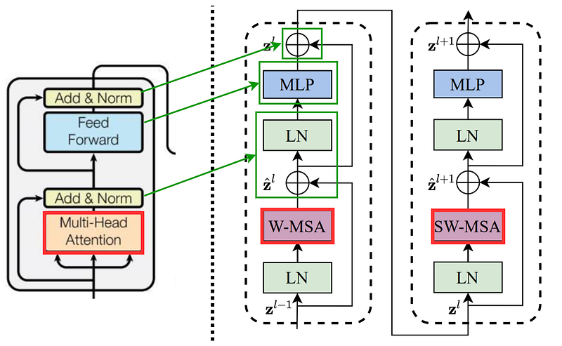
In a SWIN transformer block, two encoders are placed in series, and the output of the first encoder is fed to the second one. The first encoder computes W-MSA and the second one computed SW-MSA on the output of the first encoder. The overall architecture of a SWIN transformer🚀 block is similar to the original transformer's encoder block, except for the mechanism of computing attention. Unlike simple global MSA(multi-headed self-attention) as computed in a typical encoder block, SWIN transformer 🚀 block has W-MSA and SW-MSA.

2.6 Overall Architecture

The authors have divided the flow of an input image from a SWIN transformer into 4 stages, let’s see each one of them.

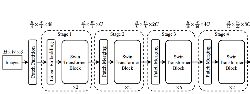
Stage 1:

1. First, an input image is passed through a patch partition, to split it into fixed-sized patches. If the image is of size H x W, and a patch is 4x4, the patch partition gives us H/4 x W/4 patches.
2. Each patch has a channel dimension, so each patch is 4x4x3 = 48 pixels. To transform each patch from 48 pixels to a better size C, we pass each patch through a linear layer (48xC), which projects each patch up to C dim, and now we have H/4 x W/4 patches, each of size C => so we have feature map of size H/4 x W/4 x C.
3. This feature map is passed through a SWIN transformer block, discussed in sec 2.4. Since the SWIN transformer block is made up of transformer encoder blocks, the size of inputs and outputs remains the same. Hence, the output of the stage-1 SWIN transformer block remains similar to the input feature map size i.e. H/4 x W/4 x C

Stage 2:

4. The feature map of size H/4 x W/4 x C, is now passed through a patch merging layer, which combines 2x2 neighboring windows and makes a new one, downsampling the resolution by 2x and increasing the feature map depth by 2. Hence H/4 x W/4 x C becomes H/8 x W/8 x 2C.

5. This feature map is passed through another SWIN transformer block, which keeps its dimensions intact.

Stage 3 and Stage 4:

6. Stage 3 and Stage 4, repeat the same procedure as stage 2, and the resolution of the feature map reduces by half after passing from each patch merging layer in each stage.

The size of feature maps at every stage is given in the above figure, which reflects that as we are going deep down in the network, the resolution of the feature map is decreasing and its depth is increasing — just like CNN! coincidence🧐 …. Nah! it’s a smart architecture choice to induce spatial inductive bias in transformers for images 😎.

That’s all folks!

In Part II, we’ll discuss how well did this SWIN transformer-based backbone, performed on benchmark datasets for object detection, image classification, and segmentation, and surprisingly was able to outperform ViT, DeIT, and SOTA convolutional networks.

Happy Learning! ❤️