Support Vector Machines (SVM) clearly explained

A Python tutorial for classification problems with 3D plots

In this article I explain the core of the SVMs, why and how to use them. Additionally, I show how to plot the support vectors and the decision boundaries in 2D and 3D.

Introduction

Everyone has heard about the famous and widely-used Support Vector Machines (SVMs). The original SVM algorithm was invented by Vladimir N. Vapnik and Alexey Ya. Chervonenkis in 1963.

SVMs are supervised machine learning models that are usually employed for classification (SVC — Support Vector Classification) or regression (SVR — Support Vector Regression) problems. Depending on the characteristics of target variable (that we wish to predict), our problem is going to be a classification task if we have a discrete target variable (e.g. class labels), or a regression task if we have a continuous target variable (e.g. house prices).

SVMs are more commonly used for classification problems and for this reason, in this article, I will only focus on the SVC models.

• NEW: After a great deal of hard work and staying behind the scenes for quite a while, we’re excited to now offer our expertise through a platform, the “Data Science Hub” on Patreon (https://www.patreon.com/TheDataScienceHub). This hub is our way of providing you with bespoke consulting services and comprehensive responses to all your inquiries, ranging from Machine Learning to strategic data analytics planning.
• Another resource. Learn Data Science and ML with the help of an 🤖 AI-powered tutor. Start here https://aigents.co/learn choose a topic and he will show up where you need him. No paywall, no signups, no ads.

Core of the method

In this article, I am not going to go through every step of the algorithm (due to the numerous amount of online resources) but instead, I am going to explain the most important concepts and terms around SVMs.

1. The decision boundary (separating hyperplane)

The SVCs aim to find the best hyperplane (also called decision boundary) that best separates (splits) a dataset into two classes/groups (binary classification problem).

Depending of the number of the input features/variables, the decision boundary can be a line (if we had only 2 features) or a hyperplane if we have more than 2 features in our dataset.

To get the main idea think the following: Each observation (or sample/data-point) is plotted in an N-dimensional space with Nbeing the number of features/variables in our dataset. In that space, the separating hyperplane is an (N-1)-dimensional subspace.

A hyperplane is an (N-1)-dimensional subspace for an N-dimensional space.

So, as stated before, for an 2-dimensional space the decision boundary is going to be just a line as shown below.

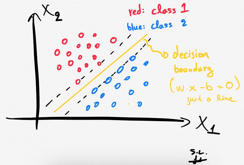
Mathematically, we can define the decision boundary as follows:

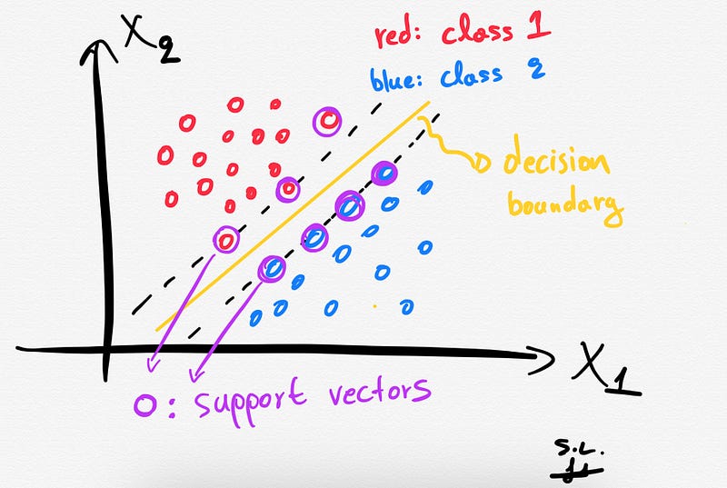
2. Support vectors

The Support vectors are just the samples (data-points) that are located nearest to the separating hyperplane. These samples would alter the position of the separating hyperplane, in the event of their removal. Thus, these are the most important samples that define the location and orientation of best decision boundary.

3. The hard margin: How does SVM find the best hyperplane?

Several different lines (or generally, different decision boundaries) could separate our classes. But which of all is the best one?

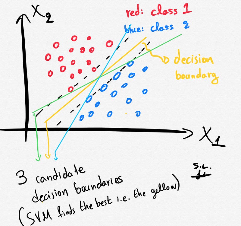
The distance between the hyperplane and the nearest data points (samples) is known as the SVM margin. The goal is to choose a hyperplane with the greatest possible margin between the hyperplane and any support vector. SVM algorithm finds the best decision boundary such as the margin is maximized. Here the best line is the yellow line as shown below.

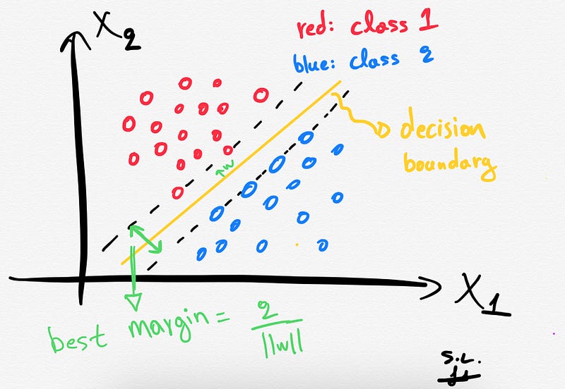
In summary, SVMs pick the decision boundary that maximizes the distance to the support vectors. The decision boundary is drawn in a way that the distance to support vectors are maximized. If the decision boundary is too close to the support vectors then, it will be sensitive to noise and not generalize well.

4. A note about the Soft margin and C parameter

Sometimes, we might want to allow (on purpose) some margin of error (misclassification). This is the main idea behind the “soft margin”. The soft margin implementation allows some samples to be misclassified or be on the wrong side of decision boundary allowing highly generalized model.

A soft margin SVM solves the following optimization problem:

• Increase the distance of decision boundary to the support vectors (i.e. the margin) and
• Maximize the number of points that are correctly classified in the training set.

It is clear that there is a trade-off between these two optimization goals. This trade-off is controlled by the famous C parameter. Briefly, if C is small, the penalty for misclassified data-points is low so a decision boundary with a large margin is chosen at the expense of a greater number of misclassifications. If C is large, SVM tries to minimize the number of misclassified samples and results in a decision boundary with a smaller margin.

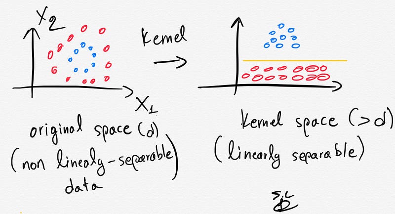
5. What happens when there is no clear separating hyperplane (kernel SVM) ?

If we have a dataset that is linearly separable then SVMs job is usually easy. However, in real life, in most of the cases we have a linearly non-separable dataset at hand and this is when the kernel trick provides some magic.

The kernel trick projects the original data points in a higher dimensional space in order to make them linearly separable (in that higher dimensional space).

Thus, by using the kernel trick we can make our non linearly-separable data, linearly separable in a higher dimensional space.

The kernel trick is based on some Kernel functions that measure similarity of the samples. The trick does not actually transform the data points to a new, high dimensional feature space, explicitly. The kernel-SVM computes the decision boundary in terms of similarity measures in a high-dimensional feature space without actually doing the projection. Some famous kernel functions include linear, polynomial, radial basis function (RBF), and sigmoid kernels.

Python working example using the Iris dataset and a linear SVC model in scikit-learn

Reminder: The Iris dataset consists of 150 samples of flowers each having 4 features/variables (i.e. sepal width/length and petal width/length).

2D

Let’s plot the decision boundary in 2D (we will only use 2 features of the dataset):

from sklearn.svm import SVC
import numpy as np
import matplotlib.pyplot as plt
from sklearn import svm, datasets

iris = datasets.load_iris()# Select 2 features / variables
X = iris.data[:, :2] # we only take the first two features.
y = iris.target
feature_names = iris.feature_names[:2]
classes = iris.target_names

def make_meshgrid(x, y, h=.02):
    x_min, x_max = x.min() — 1, x.max() + 1
    y_min, y_max = y.min() — 1, y.max() + 1
    xx, yy = np.meshgrid(np.arange(x_min, x_max, h), np.arange(y_min, y_max, h))
    return xx, yy

def plot_contours(ax, clf, xx, yy, **params):
    Z = clf.predict(np.c_[xx.ravel(), yy.ravel()])
    Z = Z.reshape(xx.shape)
    out = ax.contourf(xx, yy, Z, **params)
    return out

# The classification SVC model
model = svm.SVC(kernel="linear")
clf = model.fit(X, y)

fig, ax = plt.subplots()

# title for the plots
title = (‘Decision surface of linear SVC ‘)
# Set-up grid for plotting.
X0, X1 = X[:, 0], X[:, 1]
xx, yy = make_meshgrid(X0, X1)

plot_contours(ax, clf, xx, yy, cmap=plt.cm.coolwarm, alpha=0.8)
ax.scatter(X0, X1, c=y, cmap=plt.cm.coolwarm, s=20, edgecolors="k")
ax.set_ylabel("{}".format(feature_names[0]))
ax.set_xlabel("{}".format(feature_names[1]))
ax.set_xticks(())
ax.set_yticks(())
ax.set_title(title)
plt.show()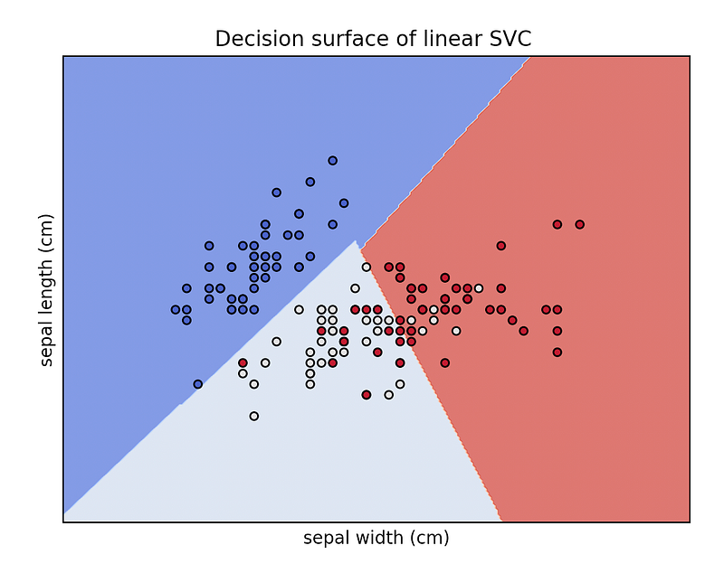

In the iris dataset, we have 3 classes of flowers and 4 features. Here we only used 2 features (so we have a 2-dimensional feature space) and we plotted the decision boundary of the linear SVC model. The colors of the points correspond to the classes/groups.

3D

Let’s plot the decision boundary in 3D (we will only use 3features of the dataset):

from sklearn.svm import SVC
import numpy as np
import matplotlib.pyplot as plt
from sklearn import svm, datasets
from mpl_toolkits.mplot3d import Axes3D

iris = datasets.load_iris()
X = iris.data[:, :3] # we only take the first three features.
Y = iris.target

#make it binary classification problem
X = X[np.logical_or(Y==0,Y==1)]
Y = Y[np.logical_or(Y==0,Y==1)]

model = svm.SVC(kernel='linear')
clf = model.fit(X, Y)

# The equation of the separating plane is given by all x so that np.dot(svc.coef_[0], x) + b = 0.

# Solve for w3 (z)
z = lambda x,y: (-clf.intercept_[0]-clf.coef_[0][0]*x -clf.coef_[0][1]*y) / clf.coef_[0][2]
tmp = np.linspace(-5,5,30)
x,y = np.meshgrid(tmp,tmp)

fig = plt.figure()
ax = fig.add_subplot(111, projection='3d')
ax.plot3D(X[Y==0,0], X[Y==0,1], X[Y==0,2],'ob')
ax.plot3D(X[Y==1,0], X[Y==1,1], X[Y==1,2],'sr')
ax.plot_surface(x, y, z(x,y))
ax.view_init(30, 60)
plt.show()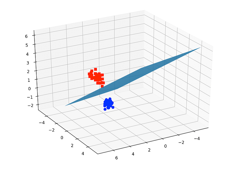

In the iris dataset, we have 3 classes of flowers and 4 features. Here we only used 3 features (so we have a 3-dimensional feature space) and only 2 classes (binary classification problem). We then plotted the decision boundary of the linear SVC model. The colors of the points correspond to the 2 classes/groups.

Plotting the support vectors

import numpy as np
import matplotlib.pyplot as plt
from sklearn import svm
np.random.seed(2)

# we create 40 linearly separable points
X = np.r_[np.random.randn(20, 2) — [2, 2], np.random.randn(20, 2) + [2, 2]]
Y = [0] * 20 + [1] * 20

# fit the model
clf = svm.SVC(kernel=’linear’, C=1)
clf.fit(X, Y)

# get the separating hyperplane
w = clf.coef_[0]
a = -w[0] / w[1]
xx = np.linspace(-5, 5)
yy = a * xx — (clf.intercept_[0]) / w[1]

margin = 1 / np.sqrt(np.sum(clf.coef_ ** 2))
yy_down = yy — np.sqrt(1 + a ** 2) * margin
yy_up = yy + np.sqrt(1 + a ** 2) * margin

plt.figure(1, figsize=(4, 3))
plt.clf()
plt.plot(xx, yy, "k-")
plt.plot(xx, yy_down, "k-")
plt.plot(xx, yy_up, "k-")

plt.scatter(clf.support_vectors_[:, 0], clf.support_vectors_[:, 1], s=80,
 facecolors="none", zorder=10, edgecolors="k")
plt.scatter(X[:, 0], X[:, 1], c=Y, zorder=10, cmap=plt.cm.Paired,
 edgecolors="k")
plt.xlabel("x1")
plt.ylabel("x2")
plt.show()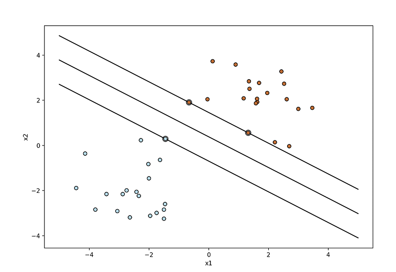

The double-circled points represent the support vectors.

• NEW: After a great deal of hard work and staying behind the scenes for quite a while, we’re excited to now offer our expertise through a platform, the “Data Science Hub” on Patreon (https://www.patreon.com/TheDataScienceHub). This hub is our way of providing you with bespoke consulting services and comprehensive responses to all your inquiries, ranging from Machine Learning to strategic data analytics planning.

Latest posts

Stay tuned & support this effort

If you liked and found this article useful, follow me! Questions? Post them as a comment and I will reply as soon as possible.

References

[1] https://www.nature.com/articles/nbt1206-1565

[1] https://en.wikipedia.org/wiki/Support_vector_machine

[2] https://scikit-learn.org/stable/modules/generated/sklearn.svm.SVC.html

Get in touch with me

• LinkedIn: https://www.linkedin.com/in/serafeim-loukas/
• ResearchGate: https://www.researchgate.net/profile/Serafeim_Loukas
• EPFL profile: https://people.epfl.ch/serafeim.loukas
• Stack Overflow: https://stackoverflow.com/users/5025009/seralouk