
How SVM constructs boundaries? Math explained.
Mathematical concepts behind how SVM can separate data points in high dimensional space

Support vector machines were first introduced by Vladmir Vapnik and his colleagues at Bell Labs in 1992. However, many are not aware that basics of support vector machines were already developed in 1960s with his PhD thesis at Moscow University. Over decades, SVM has been highly preferred by many since it uses less computational resources while allowing data scientists to achieve notable accuracy. Not to mention that it solves both classification and regression problems.
1. Basic Concept
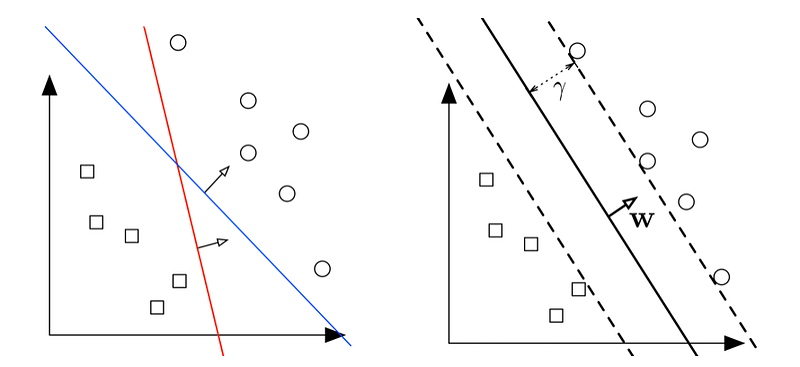
SVM can solve linear and non-linear problems and work well for many practical business problems. The principle idea of SVM is straight forward. The learning model draws a line which separates data points into multiple classes. In a binary problem, this decision boundary takes the widest street approach maximising the distance to the closest data points from each class.
In vector calculus, the dot product measures ‘how much’ one vector lies along another, and tells you the amount of force going in the direction of the displacement, or in the direction of another vector.
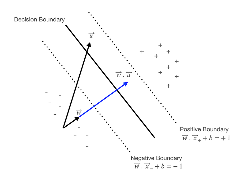
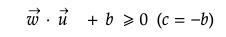
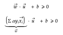
For instance, we have the unknown vector u and normal vector w which is perpendicular to the decision boundary. The dot product of w·u denotes the amount of force by u going in the direction of vector w. In this regard, if unknown vector u locates on the positive side of boundary, it can be described as below with the constant b.
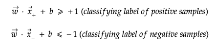
The samples locating above the boundary that classifies positive samples (+1) or below the boundary that classifies negative samples (-1) can be accordingly expressed.
2. Decision Rule — Constraint
When a decision boundary is determined, the positive and negative boundaries should be drawn in a way that the closest samples from each group maximise the width, and thus those samples are placed on each group’s boundary.
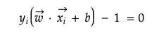
This rule will become a constraint to find the maximum width of boundaries. Given that y is +1 for positive samples and -1 for negative samples, both equations above can express sample x on the gutter of positive or negative boundary by multiplying y on both sides of equations. They are also known as support vectors. See maths explained here.
3. Decision Rule — Maximum Width
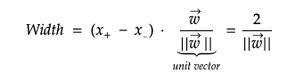
Let’s say we have the vector x+ on the gutter of positive boundary, and the vector x- on the gutter of negative boundary. The x+ minus x- stands for the directional force from the negative vector x- to the positive vector x+. If we perform dot product on this directional force with the unit vector of w which is perpendicular to the decision boundary, then this becomes the width between negative and positive boundaries. Note that w is normal vector and ||w|| is the magnitude of w. See maths explained here.
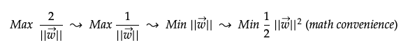
We basically maximise this width to distinctively separate negative and positive data points. This can be simplified as below. The last form squares the magnitude of w and divides it by 2 for mathematical convenience.
3. Constrained Optimisation — Find Max Width with a Constraint
The Lagrangian equation can be used to solve a constrained optimisation problem. If the constraint changes by one unit, then the maximum value of the objective function reduces by λ. The equation is generally used to find maxima or minima of the objective function given the constraints.
- L(x, λ) = f(x)- λ g(x)
- f(x): objective function
- g(x): constraint
- λ: Lagrangian
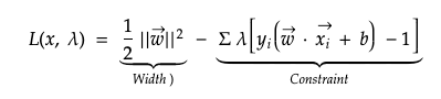
Earlier we mentioned that SVM takes the widest street approach to find the maximum width between positive and negative boundaries. This problem can be described using the Lagrangian equation with the objective function and constraint defined as below.
In summary, the Lagrangian minimises the objective function (eventually maximise the width between positive and negative boundaries) given the constraint that samples are support vectors on the gutters.
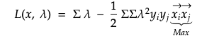
After finding the derivatives with respect to w and b from the equation above, it can be simplified as below. Since y i and y j are labels or response variables, the equation can be simply minimised by maximising the dot product of vector x i and x j. In other words, maximisation of width all depends on summing dot products of pairs of supports vectors (on the gutters) while drawing boundary lines.
Furthermore, unknown vector u is determined whether it is placed on the positive side of decision boundary depending on dot products of support vector x and u.
4. Kernel Trick
In the linear problem, SVM can easily draw a decision boundary to group samples into multiple classes. However, if data points cannot be separated with linear slices then data points can be transformed before drawing decision boundaries, which is called Kernel Trick.
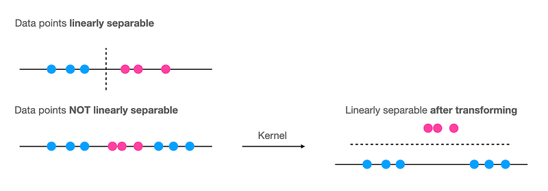
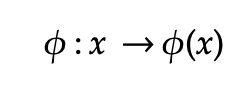
In the above, non-linear SVM becomes linear SVM problem after transforming with Kernel Trick. Kernels basically map the problem from input space to a new higher-dimensional space (called the feature space) 𝜙(x) by doing a non-linear transformation using a special function called the Kernel. Then a linear model is used to separate data points in the feature space. The linear model in the feature space corresponds to a non-linear model in the input space.
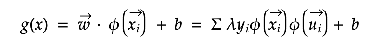
The SVM basic rule can be expressed as below in the feature space. The equation below is when the magnitude of w is replaced with linear sum of a, y and x. See maths explained here. The beauty of using Kernel is the original equation does not change since Kernel transformation is abstracted in phi 𝜙.
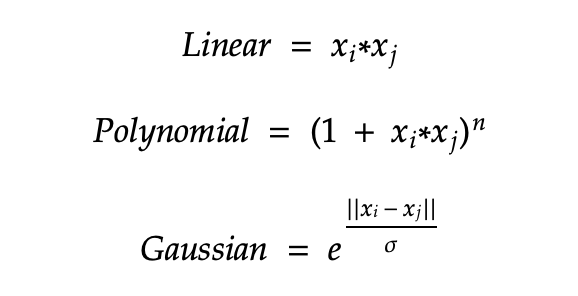
Here are examples of Kernel functions. Usually, you can start with the simplest version of transformation and gradually model with more and more advanced kernel functions to avoid overfitting.
Now that we cover how SVM solves the classification problem while drawing boundaries, we will build a model with sample dataset in the next post.
References: