Support Vector Machine: Digit Classification with Python; Including my Hand Written Digits

Understanding SVM Series : Part 3

Following the previous detailed discussions of SVM algorithm, I will finish this series with an application of SVM to classify handwritten digits. Here we will use the MNIST database for handwritten digits and classify numbers from 0 to 9 using SVM. The original data-set is complicated to process, so I am using the data-set processed by Joseph Redmon.

I have followed the Kaggle competition procedures and, you can download the data-set from the kaggle itself. The data-set is based on gray-scale images of handwritten digits and, each image is 28 pixel in height and 28 pixel in width. Each pixel has a number associated with it, where 0 represents a dark pixel and, 255 represents a white pixel. Both the train and test data-set have 785 columns where, ‘label’ column represents the handwritten digit and remaining 784 columns represent the (28, 28) pixel values. The train and test data-set contains 60,000 and 10,000 samples respectively. I will use several techniques like GridSearchCV and Pipeline which I have introduced in a previous post, and some new concepts like representing a gray-scale image in a numpy array.

I have used 12000 samples and 5000 samples from the training and test data-sets just to reduce the time of computation and it is recommended to use the full set to obtain a better score and avoid selection bias.

import math, time 
import matplotlib.pyplot as plt
import numpy as np 
import pandas as pd

start = time.time()

MNIST_train_small_df = pd.read_csv('mnist_train_small.csv', sep=',', index_col=0)
#print MNIST_train_small_df.head(3)
print MNIST_train_small_df.shape

>> (12000, 785)

We can check whether the training data-set is biased towards certain numbers or not by printing out the value_counts() and/or from the distribution plot of labels.

sns.countplot(MNIST_train_small_df['label'])
plt.show()# looks kinda okay

# or we can just print

print MNIST_train_small_df['label'].value_counts()

Figure 1: Bar plots of sample distribution in training data set

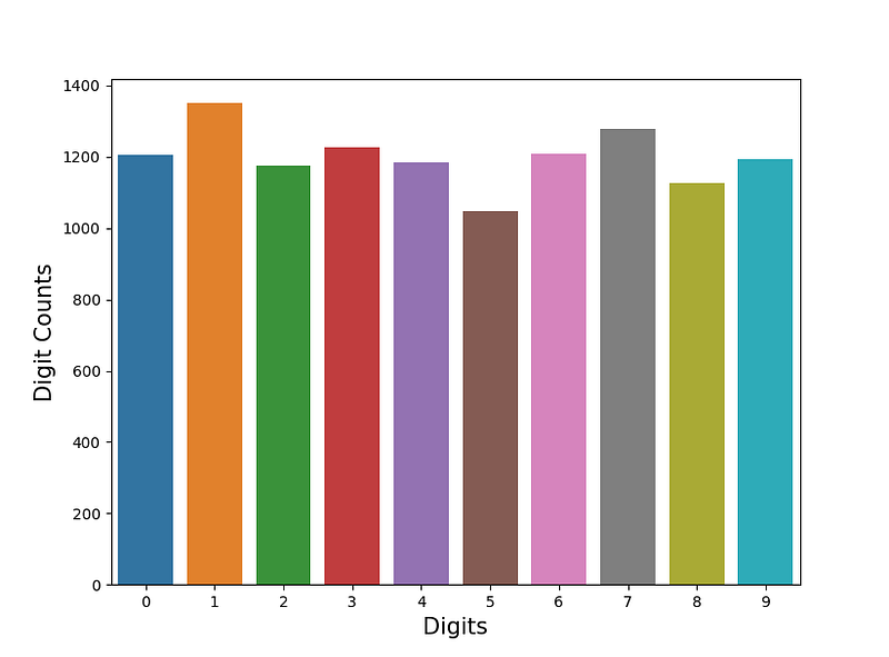
We see that selection is little biased towards digit 1 and the sample count for label 1 is around 30% higher than sample 5, and this problem persists even if we use the compete training data-set (60,000 samples). So moving on, it is time to separate label and pixel columns and, label is the 1st column of the data-frame.

X_tr = MNIST_train_small_df.iloc[:,1:] # iloc ensures X_tr will be a dataframe
y_tr = MNIST_train_small_df.iloc[:, 0]

Then I have separated training and test data with 20% samples reserved for test data. I used stratify=y to preserve distribution of labels (digits)-

X_train, X_test, y_train, y_test = train_test_split(X_tr,y_tr,test_size=0.2, random_state=30, stratify=y_tr)

As the pixel values vary in the range 0–255, it is time to use some standardization and I have used StandardScaler which standardize features by removing mean and scaling it to unit variance. Also after trying all the kernels, best score and least time is achieved with polynomial kernel. To understand more about Kernel tricks you can check the previous post.

Here we will set up the Pipeline object with StandardScaler and SVC as a transformer and estimator respectively.

steps = [('scaler', StandardScaler()), ('SVM', SVC(kernel='poly'))]
pipeline = Pipeline(steps) # define Pipeline object

To decide on the value of C, gamma we will use the GridSearchCV method with 5 folds cross-validation. If you wanna learn more about pipeline and grid-search, please check my previous post.

parameters = {'SVM__C':[0.001, 0.1, 100, 10e5], 'SVM__gamma':[10,1,0.1,0.01]}

grid = GridSearchCV(pipeline, param_grid=parameters, cv=5)

Now we are ready to test the model and find the best-fit parameters.

grid.fit(X_train, y_train)

print "score = %3.2f" %(grid.score(X_test, y_test))

print "best parameters from train data: ", grid.best_params_

>> 
score = 0.96

best parameters from train data:  {'SVM__C': 0.001, 'SVM__gamma': 10}

>>

y_pred = grid.predict(X_test)

96% accuracy is obtained with 12000 samples and I expect this score to increase a bit with the complete 60,000 samples. The GridSearchCV part is time consuming and if you want, you can directly use the C and gamma parameters.

We can check some of the predictions

print y_pred[100:105]
print y_test[100:105]

>> 
[4 2 9 6 0]
1765     4
220      2
932      9
6201     6
11636    0

We can now plot the digits using python matplotlib pyplot imshow . We use the prediction list and the pixel values from the test list for comparison.

for i in (np.random.randint(0,270,6)):
 two_d = (np.reshape(X_test.values[i], (28, 28)) * 255).astype(np.uint8)
 plt.title('predicted label: {0}'. format(y_pred[i]))
 plt.imshow(two_d, interpolation='nearest', cmap='gray')
 plt.show()

Let me briefly explain the second line of the code. As the pixel values are arranged in a row with 784 columns in the data-set, first we use numpy ‘reshape’ module to arrange it in 28 X 28 array and then multiply with 255 as the pixel values were standardized initially. Please be aware that X_test.values returns a ‘numpy’ representation of the data-frame.

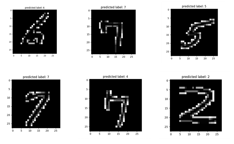
Figure 2: Examples of digit classification on training data-set.

As you can see in the images above, all of them except one was correctly classified (I think the image (1,1) is digit 7 and not 4). To know how many digits were misclassified we can print out the Confusion-Matrix. According to the definition given in scikit-learn

Confusion matrix C is such that c(i,j) is equal to the number of observations known to be in group i but predicted to be in group j.

print "confusion matrix: \n ", confusion_matrix(y_test, y_pred)

>>

[[236   0   0   1   1   2   1   0   0   0]
 [  0 264   1   1   0   0   1   1   2   0]
 [  0   1 229   1   2   0   0   0   1   1]
 [  0   0   2 232   0   3   0   2   5   2]
 [  0   1   0   0 229   1   1   0   1   4]
 [  0   0   1   4   1 201   0   0   1   2]
 [  3   1   2   0   3   3 229   0   0   0]
 [  0   1   3   0   6   0   0 241   0   5]
 [  0   0   3   6   1   2   0   0 213   0]
 [  3   1   1   0   1   0   0   1   2 230]]

So if we consider the 1st row, we can understand that out of 241 zeros, 236 were correctly classified and so on..

Now we will repeat the process for the test-data set (mnist_test.csv) but instead of going through finding the best parameters for SVM (C, gamma) using GridSearchCV , I have used the same parameters from the training data set.

I have used 5000 samples instead of 10,000 test samples to reduce time consumption, as mentioned before.

MNIST_df = pd.read_csv('mnist_test.csv')
MNIST_test_small = MNIST_df.iloc[0:5000]
MNIST_test_small.to_csv('mnist_test_small.csv')
MNIST_test_small_df = pd.read_csv('mnist_test_small.csv', sep=',', index_col=0)

Next step is choosing features and labels —

X_small_test = MNIST_test_small_df.iloc[:,1:]
Y_small_test = MNIST_test_small_df.iloc[:,0]

Divide the features and labels into train and test sets

X_test_train, X_test_test, y_test_train, y_test_test = train_test_split(X_small_test,Y_small_test,test_size=0.2, random_state=30, stratify=Y_small_test)

Set up the Pipeline object

steps1 = [('scaler', StandardScaler()), ('SVM', SVC(kernel='poly'))]
pipeline1 = Pipeline(steps1) # define

Set up GridSearchCV object but this time we use the parameters estimated using the mnist_train.csv file.

parameters1 = {'SVM__C':[grid.best_params_['SVM__C']], 'SVM__gamma':[grid.best_params_['SVM__gamma']]}

grid1 = GridSearchCV(pipeline1, param_grid=parameters1, cv=5)
grid1.fit(X_test_train, y_test_train)

print "score on the test data set= %3.2f" %(grid1.score(X_test_test, y_test_test))

print "best parameters from train data: ", grid1.best_params_ # same as previous with training data set

>>
score on the test data set= 0.93

best parameters from train data:  {'SVM__C': 0.001, 'SVM__gamma': 10}

>>

y_test_pred = grid1.predict(X_test_test)

Score on the test data set is 93% compared to the score of 96% on train data set. Below are some of the random images from the test data set compared with the predicted level.

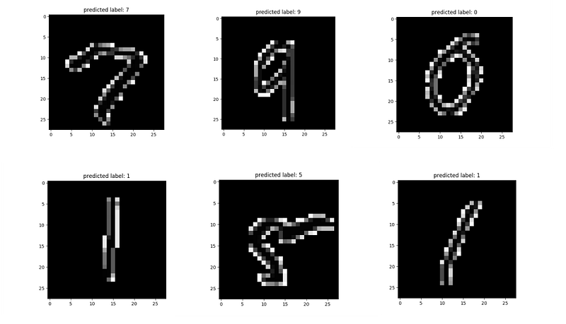
Figure 3: Examples of digit classification on test data-set.

We can check the confusion matrix for the test data-set to have an overall view of misclassification.

print "confusion matrix: \n ", confusion_matrix(y_test_test, y_test_pred)

>>

[[ 91   0   0   0   0   0   0   0   1   0]
 [  0 111   2   0   1   0   0   0   0   0]
 [  0   0  98   1   0   0   1   2   4   0]
 [  0   0   1  91   0   2   0   0   4   2]
 [  0   0   0   1  95   0   0   1   0   3]
 [  0   0   1   3   1  77   4   0   3   2]
 [  1   1   1   0   2   0  85   0   2   0]
 [  0   0   0   1   0   0   0 100   0   2]
 [  0   0   1   1   0   2   0   1  93   0]
 [  0   0   0   0   4   1   0   3   3  93]]

Notice that there’s just only 1 misclassification in digit 0 out of 92 labels. Now we will move on to discuss the possibility of classifying my own hand-written images.

Classifying Own Hand-Written Images:

Below are the steps I have taken to prepare the data-set and then classify digits starting from 0 to 9

I’ve used mypaint to first write (paint) images and and then used Imagemagick to resize images with height and width of 28X28 pixels.

convert -resize 28X28! sample_image0.png sample_image0_r.png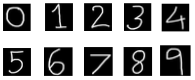

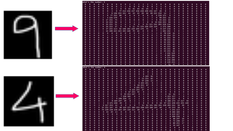
Figure 4: Resized (28X28) My Own Hand-written Images

2. Converting an image to numpy array and check how the pixel values are distributed. You can find the code on my github and below are 2 examples —

Figure 5: Representing images with pixels using Image and Numpy

3. Flatten the array (28X28) to (784,) and convert it to to a list. Then write it on a csv file including label i.e. the digits the pixels represent. So total number columns now is 785, in consistence with the train and test csv files that I have used before. The codes are available in github.com.

4. Concatenate the new data-frame with the test data-frame, So that the new file now have 10 more rows.

5. Finally run the same classification process with this new file, with only one difference — train and test data are not prepared using train_test_split method as my primary intention is to see how the algorithm works on the new data. So I have chosen first 3500 rows for training and remaining rows (including the new data) as test samples.

X_hand_train = new_file_df_hand.iloc[0:3500, 1:]
X_hand_test  = new_file_df_hand.iloc[3500:5011, 1:]
y_hand_test = new_file_df_hand.iloc[3500:5011, 0]
y_hand_train = new_file_df_hand.iloc[0:3500, 0]

6. To plot the hand-written images and how well they matches with the predicted output, I have used the following for loop as before — Since last 1500 samples including my own handwritten images are taken as test data, the loop is over final few rows.

for ik in range(1496, 1511, 1):
 three_d = (np.reshape(X_hand_test.values[ik], (28, 28)) * 255).astype(np.uint8)
 plt.title('predicted label: {0}'. format(y_hand_pred[ik]))
 plt.imshow(three_d, interpolation='nearest', cmap='gray')
 plt.show()

7. The score on the test data-set including my own hand-written data is 93% .

8. Let’s look at how well the classifier the could classify my handwriting from 0 to 9

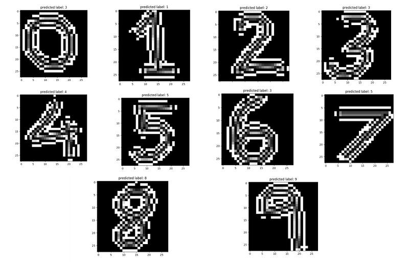
Figure 5: Predicted labels on my hand-written digits. 70% correct !!!

So 7 out of 10 hand-written digits were correctly classified and that’s great because if you compare with the MNIST database images, my own images are different and I think one reason is the choice of brush. As I realized, the brush I have used, produced much thicker images. Especially while comparing with the MNIST images, I see between the edges the pixels are brighter (higher pixel values — > 255 ) in my images compared with the MNIST images and that could be reason of 30% misclassification.

I guess you have got an idea how to use Support Vector Machine to deal with more realistic problems. As a mini project you can use similar algorithm to classify MNIST fashion data.

Hopefully you have enjoyed the post, and to learn more about the fundamentals about SVM please check my previous posts in this series.