Strategies for Balancing Multiple Loss Functions in Deep Learning

In many deep learning tasks, training models often involves balancing various objectives. For instance, when training a model for low-light image enhancement, it is crucial to improve the overall lighting (loss function 1) while maintaining the natural distribution of colors (loss function 2). The challenge lies in effectively minimizing multiple losses together. This article introduces methods for balancing multiple loss functions during the training of deep learning models and provides some sample code for better understanding.

Let us consider n loss functions:

Each loss function can be viewed as a separate task, and therefore optimizing multiple loss functions can be viewed as multi-task learning. Our goal is to minimize each loss function as much as possible.

1. Transform to single-task learning

A straightforward idea is to introduce weights and transform multi-task learning into a single-task learning by weighted summation as follows:

the question now is how to determine each weight. In the following, we assume that each task is supposed to be treated equally. If not, then additional weights can be added on top of the methods described below to reflect the priority of task according to your domain knowledge. In the absence of task priors and biases, the most natural choice would be setting all weights to 1/n .

However, in reality, each task can differ significantly. For instance, mixing tasks with different numbers of categories in classification, combining classification and regression tasks, or integrating classification and generative tasks. Each loss function may have different magnitudes, making their direct summation meaningless.

1.1 Use Initial Loss Value

One approach is to use the reciprocal of the initial value of each loss function as its weight, namely

since each loss is divided by its own initial value, larger losses will be scaled down, while smaller losses will be amplified, thus approximately balancing each loss.

So, how can we estimate the initial loss for each task? The most straightforward method is to use a few batches of data to estimate it. Beyond this, we can derive a theoretical value based on some assumptions. For instance, under common initialization practices, we can assume that the output of the initial model (before activation functions) is a zero vector. If a softmax is added, the distribution becomes uniform. Therefore, for a “K-class classification + cross-entropy” problem, the initial loss would be log(K) . for a “regression + L2 loss” problem, the initial loss can be estimated using a zero vector, i.e.

where D represents the complete set of training labels.

1.2 Use Prior Loss Value

One issue with using the initial loss is that the initial state might not accurately reflect the learning difficulty of the current task. A better approach could be to change “initial state” to “prior state”.

For example, in K-class classification, if the frequency of each class is [p_1, p_2, …, p_K] (prior distribution), although the initial state’s prediction distribution is uniform, we can reasonably assume that the model can easily learn to predict the outcome of each sample as [p_1, p_2, …, p_K]. In this case, the model’s loss would be entropy:

In a sense, the “prior distribution” better captures the essence of “initial” than the “initial distribution.” It represents the notion that “even if the model learns nothing, it knows to produce results randomly according to the prior distribution.” Therefore, the loss value at this state more accurately represents the initial difficulty of the current task. Hence, using prior loss value​ instead of initial loss value should be more reasonable. Similarly, for the “regression + L2 loss” problem, the prior outcome should be the expectation of all labels,

Thus, we can use

hoping to achieve better results.

1.3 Use Real-time Loss Value

In 1.1 and 1.2, the core idea is to use the reciprocal of the loss values as task weights. We can also simply use the reciprocal of “real-time” loss values to dynamically adjust the weights. Specifically,

For instance, we can implement this idea using one line of code in Pytorch:

# Normalizing losses and combining them
combined_loss = loss_1 / loss_1.detach() + loss_2 / loss_2.detach()

# Backpropagation
combined_loss.backward()

In this approach, the loss function for each task is adjusted to always equal 1, ensuring consistent magnitudes. Due to the presence of the detach operation, although the loss is constantly 1, its gradient is not always zero:

Simply put, after detach a loss from computation graph, we can treat the detached loss as a constant. Thus, the final result dynamically adjusts the gradient proportions using the latest loss value​. Many experiments have demonstrated that this approach can indeed serve as a quite effective baseline in most situations.

1.4 Weighting Via Uncertainty

In 1.3, we have introduced two dynamic ways to update weights. In [2], the authors proposed another way to dynamically update weights, where homoscedastic uncertainty is used to balance the single-task losses. The homoscedastic uncertainty or task-dependent uncertainty is not an output of the model, but a quantity that remains constant for different input examples of the same task.

Assume we have two tasks, and both follow a Gaussian distributions (which is common for regression tasks, for classification tasks the final formulation is pretty similar, please refer to the original paper [2] if you are interested):

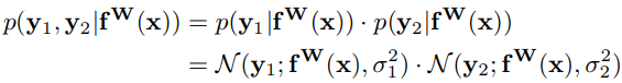
The optimization procedure is carried out to maximize a Gaussian likelihood objective that accounts for the homoscedastic uncertainty. In particular, they optimize the model weights W and the noise parameters σ1, σ2 to minimize the following objective:

By minimizing the loss L w.r.t. the noise parameters σ1, σ2, one can essentially balance the task-specific losses during training. The optimization objective above can easily be extended to account for more than two tasks. The noise parameters are updated through standard back-propagation during training.

The last term logσ1σ2 can be viewed as a penalty term. From the penalty perspective, to avoid negative penalty during training, we can modify log(σ) to log(1+σ²). Here is a PyTorch example:

import torch
import torch.nn as nn

class AutomaticWeightedLoss(nn.Module):
    """
    Automatically weighted multi-task loss.

    Params:
        num: int
            The number of loss functions to combine.
        x: tuple
            A tuple containing multiple task losses.

    Examples:
        loss1 = 1
        loss2 = 2
        awl = AutomaticWeightedLoss(2)
        loss_sum = awl(loss1, loss2)
    """
    def __init__(self, num=2):
        super(AutomaticWeightedLoss, self).__init__()
        # Initialize parameters for weighting each loss, with gradients enabled
        params = torch.ones(num, requires_grad=True)
        self.params = nn.Parameter(params)

    def forward(self, *losses):
        """
        Forward pass to compute the combined loss.

        Args:
            *losses: Variable length argument list of individual loss values.

        Returns:
            torch.Tensor: The combined weighted loss.
        """
        loss_sum = 0
        for i, loss in enumerate(losses):
            # Compute the weighted loss component for each task
            weighted_loss = 0.5 / (self.params[i] ** 2) * loss
            # Add a regularization term to encourage the learning of useful weights
            regularization = torch.log(1 + self.params[i] ** 2)
            # Sum the weighted loss and the regularization term
            loss_sum += weighted_loss + regularization

        return loss_sum

2. Manipulate Gradient of Each Loss

2.1 Gradient normalization

All four methods above only consider scale the loss functions. However, the gradient of each loss may not have the similar magnitude. The paper GradNorm [6] proposed to control the training of multi-task networks by pushing the task-specific gradients to be of similar magnitude. By doing so, the network is encouraged to learn all tasks at an equal pace. The weights are time varying in GradNorm, the weighted loss at iteration t can be written as:

Let’s introduce some notations before moving on:

GradNorm wants to establish a common scale for gradient magnitudes, and balance training rates of different tasks (i.e., r_i(t) defined above). To achieve the goal, the objective is set as minimizing:

The weights for losses (NOT the weights of neural networks) are updated as

The network weights W is generally chosen as the last shared layer of weights to save on compute costs, instead of using all layers. Here is a sample code for implementing GradNorm in Pytorch:

import torch
import torch.nn as nn
import torch.optim as optim

class GradNormLoss(nn.Module):
    def __init__(self, num_of_task, alpha=1.5):
        super(GradNormLoss, self).__init__()
        self.num_of_task = num_of_task  # Total number of tasks
        self.alpha = alpha  # Alpha value for adjusting relative losses
        self.w = nn.Parameter(torch.ones(num_of_task, dtype=torch.float))  # Task-specific weights
        self.l1_loss = nn.L1Loss()  # L1 Loss for regularization
        self.L_0 = None  # Reference to initial losses for each task

    def forward(self, L_t: torch.Tensor):
        """ Compute the total weighted loss for the tasks. """
        # Initialize the initial losses `Li_0` if not already done
        if self.L_0 is None:
            self.L_0 = L_t.detach()  # Detach to prevent gradients
        # Compute the weighted losses `w_i(t) * L_i(t)`
        self.wL_t = L_t * self.w
        # Sum up the weighted losses
        self.total_loss = self.wL_t.sum()
        return self.total_loss

    def additional_forward_and_backward(self, grad_norm_weights: nn.Module, optimizer: optim.Optimizer):
        """ Perform additional forward and backward pass to adjust task weights. 
            grad_norm_weights: the layers for computing gradients
            optimizer: optimizer for updating weights of losses      
        """
        # Perform standard backward pass on the total loss
        self.total_loss.backward(retain_graph=True)
        # Reset gradients for task weights as they shouldn't be updated in this pass
        self.w.grad.zero_()

        # Calculate the gradients of the loss w.r.t. the shared parameters and their norms
        GW_t = [torch.norm(torch.autograd.grad(
                self.wL_t[i], grad_norm_weights.parameters(), retain_graph=True, create_graph=True)[0])
                for i in range(self.num_of_task)]
        self.GW_t = torch.stack(GW_t)  # Stack to create a single tensor

        # Calculate average gradient norms
        self.bar_GW_t = self.GW_t.mean().detach()
        # Calculate normalized losses and relative inverse training rates
        self.tilde_L_t = (L_t / self.L_0).detach()
        self.r_t = self.tilde_L_t / self.tilde_L_t.mean()
        # Calculate the gradient normalization loss
        grad_loss = self.l1_loss(self.GW_t, self.bar_GW_t * (self.r_t ** self.alpha))

        # Compute gradients for the task weights
        self.w.grad = torch.autograd.grad(grad_loss, self.w, only_inputs=True)[0]
        # Update weights using optimizer
        optimizer.step()

        # Re-normalize weights to keep their sum constant
        self.w.data = self.w.data / self.w.data.sum() * self.num_of_task

        # Clear intermediate variables to free memory
        self.GW_t, self.bar_GW_t, self.tilde_L_t, self.r_t, self.wL_t = None, None, None, None, None

As a side note:

As GradNorm aims to balance the gradients of different losses to have a similar scale, one might ask, “Why not directly normalize the gradient of each loss?” That is:

or even further, add rate adjustment as GradNorm did:

Although I have not tried, this could be a worthwhile approach to explore :)

2.2 Gradient Surgery for Alleviating Task Conflicting

Learning multiple tasks all at once results is a difficult optimization problem, sometimes leading to worse overall performance and data efficiency compared to learning tasks individually. In [7], the authors identified a set of three conditions of the multi-task optimization landscape that cause detrimental gradient interference, and hypothesize that one of the main optimization issues in multi-task learning arises from gradients from different tasks conflicting with one another in a way that is detrimental to making progress. To resolve the issue, [7] proposed a method called PCGrad.

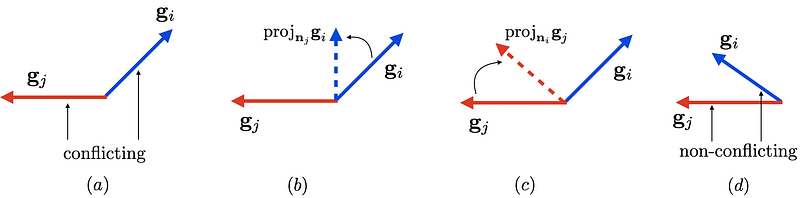
The figure above shows conflicting gradients and PCGrad. In (a), tasks i and j have conflicting gradient directions, which can lead to destructive interference. (b) and (c) illustrate the PCGrad algorithm in the case where gradients are conflicting. PCGrad projects task i’s gradient onto the normal vector of task j’s gradient, and vice versa. Non-conflicting task gradients (d) are not altered under PCGrad. The pseudo code of PCGrad is shown below.

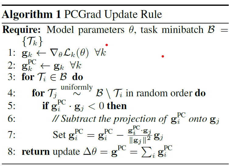
Here is a PyTorch example for PCGrad from this repo:

    def _project_conflicting(self, grads, has_grads, shapes=None):
        shared = torch.stack(has_grads).prod(0).bool()
        pc_grad, num_task = copy.deepcopy(grads), len(grads)
        for g_i in pc_grad:
            random.shuffle(grads)
            for g_j in grads:
                g_i_g_j = torch.dot(g_i, g_j)
                if g_i_g_j < 0:
                    g_i -= (g_i_g_j) * g_j / (g_j.norm()**2)
        merged_grad = torch.zeros_like(grads[0]).to(grads[0].device)
        if self._reduction:
            merged_grad[shared] = torch.stack([g[shared]
                                           for g in pc_grad]).mean(dim=0)
        elif self._reduction == 'sum':
            merged_grad[shared] = torch.stack([g[shared]
                                           for g in pc_grad]).sum(dim=0)
        else: exit('invalid reduction method')

        merged_grad[~shared] = torch.stack([g[~shared]
                                            for g in pc_grad]).sum(dim=0)
        return merged_grad

3. From Pareto Optimal Perspective

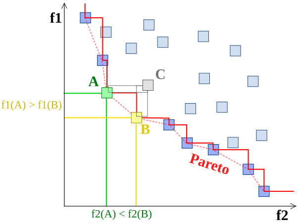
Due to the complex nature of multi-task learning, a certain choice that improves the performance for one task could lead to performance degradation for another task as shown in 2.2. The loss balancing methods discussed beforehand try to tackle this problem by setting the task-specific weights or modifying task gradients. Differently, the authors in [3] view multi-task learning as a multi-objective optimization problem, with the overall goal of finding a Pareto optimal solution among all tasks.

A Pareto optimal solution is found when the following condition is satisfied: the loss for any task can be decreased without increasing the loss on any of the other tasks.

Let’s consider the 1st order expansion of single-task loss function:

If the inner product between the loss gradient and the parameters update direction is negative:

then the loss can be (approximately) decreased. The Δθ is simply gradient descent direction.

Seeking Pareto optimal means we need to find a direction -Δθ that satisfies:

We are primarily concerned with whether there exists a non-zero solution in the feasible region: if there is one, then we identify it as the direction for updates; if there is none, it is possible that Pareto optimality has been reached (necessary but not sufficient), and we refer to this state as a Pareto Stationary Point. To simplify the notation, we denote gradient as:

Then, one observation is

So we just need to maximize the minimum of those ⟨g_i, u⟩, then we can obtain a good update direction u as -Δθ. The problem now becomes:

However, once there exists a non-zero u such that mini⟨g_i, u⟩>0, then letting the magnitude of u approach positive infinity, the maximum value will tend towards positive infinity. Therefore, for the stability of the result, we need to add a regularization term and consider the following object instead:

Now, we define the set of weights for each (single-task) loss (or say weights for each gradient) as:

and it is easy to verify:

so the objective (1) is equivalent to:

The above function is concave with respect to u and convex with respect to α, and the feasible regions for both u and α are convex sets (the weighted average of any two points in the set still lies within the set). Therefore, according to Minimax Theorem, the min and max can be interchanged:

The right side of the equation is because the max part is just an unconstrained quadratic function maximization problem, which can directly computed and obtain the best u:

Therefore, only the min part remains, and the problem becomes finding a weighted average of gradients such that its magnitude is minimized.

In [3], the authors proposed to use Frank-Wolfe algorithm to solve (2). The Frank-Wolfe algorithm is an iterative first-order optimization algorithm which contains 3 steps in each iteration:

Step 1. Linearize the object using first-order approximation (around α^k, i.e., the solution from the previous iteration) and find the solution for the sub-problem:

Step 2. Use the solution from step 1 as direction, find a step size, which can be calculated explicitly (refer to [3])

Step 3. Update solution

Simply put, the Frank-Wolfe algorithm first finds the direction for the next update. Then, it performs an interpolation search between α and e_τ, finding the optimal solution as the result of the iteration.

As you can see, this method is more complicated compared to other methods introduced in previous sections. If you are interested in Pytorch implementation, please refer to this github repository.

Conclusion

So far, we have covered six methods for optimizing multiple losses simultaneously. It is important to note that these methods may not always be effective, and you may need to conduct necessary tests and adjustments for your specific problem. I hope you enjoy reading!

References:

1. 多任务学习漫谈 (1 and 2) https://spaces.ac.cn/archives/8896
2. Multi-Task Learning Using Uncertainty to Weigh Losses for Scene Geometry and Semantics (ICCV 2018)
3. Multi-task learning as multi-objective optimization (NeurIPS 2018)
4. Multi-Task Learning for Dense Prediction Tasks: A Survey
5. https://github.com/Mikoto10032/AutomaticWeightedLoss
6. GradNorm: Gradient Normalization for Adaptive Loss Balancing in Deep Multitask Networks (ICML 2018)
7. Gradient Surgery for Multi-Task Learning (NeurIPS 2020)