Stock predictions with state-of-the-art Transformer and Time Embeddings

Feeding a trading bot with state-of-the-art stock predictions

In my previous post, I have shared my first research results for predicting stock prices which will be subsequently used as input for a deep learning trading bot. While upscaling my datasets to thousands of equity tickers equating to almost 1 Terabyte of stock price histories and news articles, I have come to realize that my initial approach of working with neural networks that are comprised of LSTM(Long-Short Term Memory Models) and CNN (Convolutional Neural Network) components has its limitations. Thus, to overcome the limitations I had to implement a Transformer, specialized for stock time-series.

In recent years Transformers have gained popularity due to their outstanding performance. Combining the self-attention mechanism, parallelization, and positional encoding under one hood provides usually an edge over classical LSTM and CNN models when working on tasks where semantic feature extraction and large datasets are required [1].

Since I was not able to find a simple Transformer implementation which is customized for time-series sequences that have multiple features e.g. the (Open, High, Low, Close, Volume) features of our stock data I had to implement it myself. In this post, I’ll be sharing my Transformer architecture for stock data as well as what Time Embeddings are and why it essential to use them in combination with time-series.

Data

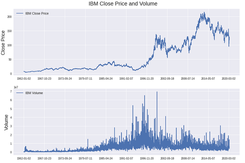
For the explanatory purpose of this article, we will be using the IBM stock price history as a simplified version of the 1 Terabyte stock dataset. Nonetheless, you can easily apply to code in this article to a significantly larger dataset. The IBM dataset starts on the 1962–01–02, ends on the date 2020–05–24 and contains in total 14699 trading days. Additionally, for every training day, we have the Open, High, Low, and Close price as well as the trading Volume (OHLCV) of the IBM stock.

Data preparation

The price and volume features are converted into daily stock returns and daily volume changes, a min-max normalized is applied and the time-series is split into a training, validation, and test set. Converting stock prices and volumes into daily change rates increases the stationarity of our dataset. Thus the learnings a model derives from our dataset have a higher validity for future predictions. Here an overview of how the transformed data looks like.

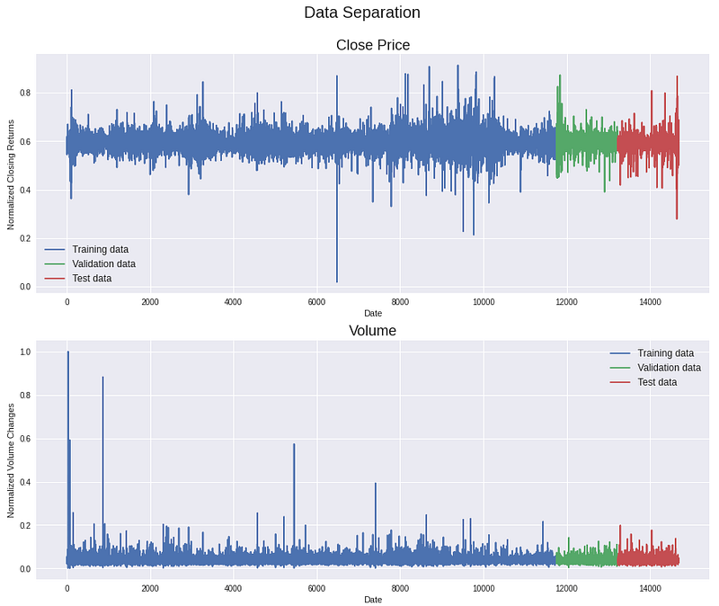
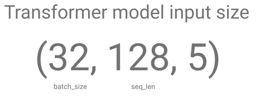
Lastly, the training, validation, and test sets are separated into individual sequences with a length of 128 days each. For each sequence day, the 4 price features (Open, High, Low, Close) and the Volume feature are present, resulting in 5 features per day. During a single training step, our Transformer model will receive 32 sequences (batch_size = 32) that are 128 days long (seq_len=128) and have 5 features per day as input.

Time Embeddings

As the first step of our Transformer implementation, we have to consider how to encode the notion of time which is hidden in our stock prices into our model.

When processing time-series data, time is an essential feature. However, when processing time-series/sequential data with a Transformer, sequences are forwarded all at once through the Transformer architecture, making it difficult to extract temporal/sequential dependencies. Thus, Transformers that are used in combination with natural language data tend to utilize positional encoding to provide a notion of word order to the model. In detail, the positional encoding is a representation of a word’s value and its position in a sentence, allowing the Transformer to obtain knowledge about a sentence structure and word interdependencies. An example of positional encoding can be found when looking under the hood of the BERT [2] model, which has achieved state-of-the-art performance for many language tasks.

Similarly, a Transformer requires a notion of time when processing our stock prices. Without Time Embeddings, our Transformer would not receive any information about the temporal order of our stock prices. Hence, a stock price from 2020 can have the same influence on tomorrows’ price prediction as a price from the year 1990. And of course, this would be ludicrous.

Time2Vector

In order to overcome a Transformer’s temporal indifferences, we will implement the approach described in the paper Time2Vec: Learning a Vector Representation of Time [2]. The authors of the paper propose “a model-agnostic vector representation for time, called Time2Vec”. You can think of a vector representation just like a normal embedding layer that can be added to a neural network architecture to improve a model’s performance.

Boiling the paper down to its essentials, there are two main ideas to consider. Firstly, the authors identified that a meaningful representation of time has to include both periodic and non-periodic patterns. An example of a periodic pattern is the weather that varies over different seasons. In contrast, an example of a non-periodic pattern would be a disease, which occurs with a high probability, the older a patient.

Secondly, a time representation should have an invariance to time rescaling, meaning that the time representation is not affected by different time increments e.g. (days, hours or seconds) and long time horizons.

Combining the ideas of periodic and non-periodic patterns as well as the invariance to time rescaling we are presented by the following mathematical definition. No worries, it is easier than it looks and I’ll explain it in detail. 😉

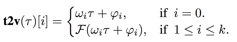
The time vector/representation t2v is comprised of two components, where ωᵢτ + φᵢ represents the non-periodic/linear and F(ωᵢτ + φᵢ) the periodic feature of the time vector.

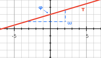
Rewriting t2v(τ) = ωᵢτ + φᵢ in a simpler way, the new version y = mᵢx + bᵢ should look familiar since it is the vanilla version of a linear function that you know from high school. ω in ωᵢτ + φᵢ is a matrix that defines the slope of our time-series τ and φ in simple terms is a matrix that defines where our time-series τ intersects with the y-axis. Hence, ωᵢτ + φᵢ is nothing more than a linear function.

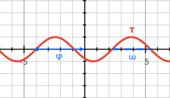
The second component F(ωᵢτ + φᵢ) represents the periodic feature of the time vector. Just like before we have the linear term ωᵢτ + φᵢ again, however, this time the linear function is wrapped in an additional function F(). The authors experimented with different functions to best describe a periodic relationship (sigmoid, tanh, ReLU, mod, triangle, etc.). In the end, a sine-function achieved the best and most stable performance (cosine achieved similar results). When combining the linear function ωᵢτ + φᵢ with a sine function the 2D representation looks as follows. φ shifts the sine function along the x-axis and ω determines the wavelength of the sine function.

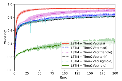
Let’s have a look at an overview of how the accuracy of an LSTM network in combination with different non-linear functions of the time vector (Time2vec) changes. We can clearly see that the ReLU function performs the worst, in contrast, the sine function outperforms every other non-linear function. The reason, the ReLU function has such an unsatisfying results is that a ReLU function is not invariant to time rescaling. The higher the invariant of a function to time rescaling the better the performance.

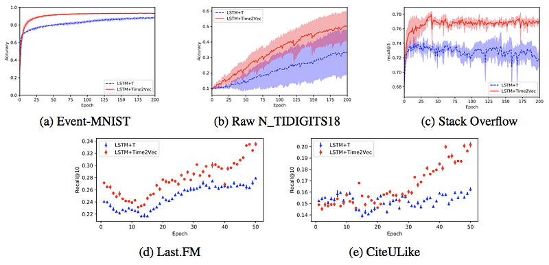
Time2Vector performance improvement

Before we start implementing the time embedding let’s take look at the performance difference of a normal LSTM network (blue) and an LSTM+Time2Vec network (red). As you can see the proposed time vector leads across multiple datasets never to worse performance and almost always improves a model’s performance. Equipped with these insights we move on to the implementation.

Time2Vector Keras implementation

Ok, we have discussed how the periodic and non-periodic components of our time vector work in theory, now we’ll implement them in code. In order for the time vector to be easily integrated in any kind of neural network architecture, we’ll define the vector as a Keras layer. Our custom Time2Vector Layer has two sub-functions def build(): and def call():. In def build(): we initiate 4 matrices, 2 for ω and 2 forφ since we need aω and φ matrix for both non-periodical (linear) and the periodical (sin) features.

seq_len = 128

def build(input_shape):
   weights_linear = add_weight(shape=(seq_len), trainable=True)
   bias_linear = add_weight(shape=(seq_len), trainable=True)

   weights_periodic = add_weight(shape=(seq_len), trainable=True)
   bias_periodic = add_weight(shape=(seq_len), trainable=True)

After having initiated our 4 matrices we define the calculation steps that will be performed once the layer is called, hence the def call(): function.

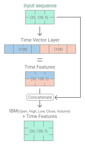
The input which will be received by the Time2Vector layer has the following shape (batch_size, seq_len, 5) → (32, 128, 5). The batch_size defines how many stock price sequences we want to feed into the model/layer at once. The seq_len parameter determines the length of a single stock price sequence. Lastly, the number 5 is derived from the fact that we have 5 features of the daily IBM stock recording (Open price, High price, Low price, Close price, Volume).

The first calculation step excludes the Volume and takes an average across the Open, High, Low, and Close prices, resulting in the shape (batch_size, seq_len) .

x = tf.math.reduce_mean(x[:,:,:4], axis=-1)

Next, we calculate the non-periodic (linear) time feature and expand the dimension by 1 again. (batch_size, seq_len, 1)

time_linear = weights_linear * x + bias_linear

time_linear = tf.expand_dims(time_linear, axis=-1)

The same process is repeated for the periodic time feature, also resulting in the same matrix shape. (batch_size, seq_len, 1)

time_periodic = tf.math.sin(tf.multiply(x, weights_periodic) + bias_periodic)

time_periodic = tf.expand_dims(time_periodic, axis=-1)

The last step that is needed to conclude the time vector calculation is concatenating the linear and periodic time feature. (batch_size, seq_len, 2)

time_vector = tf.concat([time_linear, time_periodic], axis=-1)

Time2Vector layer

Combining all steps into one Layer function the code looks as follows.

Transformer

Now we know that it is important to provide a notion of time and how to implement a time vector, the next step will be the Transformer. A Transformer is a neural network architecture that uses a self-attention mechanism, allowing the model to focus on the relevant parts of the time-series to improve prediction qualities. The self-attention mechanism consists of a Single-Head Attention and Multi-Head Attention layer. The self-attention mechanism is able to connect all time-series steps with each other at once, leading to the creation of long-term dependency understandings. Finally, all these processes are parallelized within the Transformer architecture, allowing an acceleration of the learning process.

Combining IBM data and time features — Feeding the Transformer

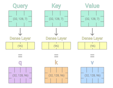
After having implemented the Time Embeddings we will be using the time vector in combination with IBM’s price and volume features as input for our Transformer. The Time2Vector layer receives the IBM price and volume features as input and calculates the non-periodic and periodic time features. In the subsequent model step, the calculated time features are concatenated with the price and volume features forming a matrix, with the shape (32, 128, 7).

Single-Head Attention

The IBM time-series plus the time features which we just calculated, form the initial input to the first single-head attention layer. The single-head attention layer takes 3 inputs (Query, Key, Value) in total. For us, each Query, Key, and Value input is representative of the IBM price, volume, and time features. Each Query, Key, and Value input receives a separate linear transformation by going through individual dense layers. Providing the dense layers with 96 output cells was a personal architectural choice.

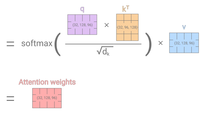
After the initial linear transformation, we will calculate the attention score/weights. The attention weights determine how much focus is placed on individual time-series steps when predicting a future stock price. Attention weights are calculated by taking the dot-product of the linearly transformed Query and Key inputs, whereas the transformed Key input has been transposed to make the dot-product multiplication feasible. Then the dot-product is divided by the dimension size of the previous dense layers (96), to avoid exploding gradients. The divided dot-product then goes through the softmax function to yield a set of weights that sum up 1. As the last step, the calculated softmax matrix which determines the focus of each time step is multiplied with the transformed v matrix which concludes the single-head attention mechanism.

Since illustrations are great for first initial learnings but lack the implementation aspect, I have prepared a clean SingleAttention Keras layer function for you guys 🙂.

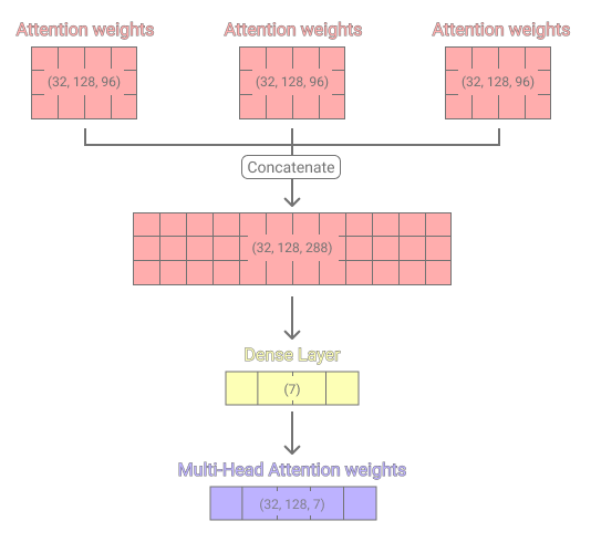
Multi-Head Attention

To further improve the self-attention mechanism the authors of the paper Attention Is All You Need [4] proposed the implementation of multi-head attention. The functionality of a multi-head attention layer is to concatenate the attention weights of n single-head attention layers and then apply a non-linear transformation with a Dense layer. The illustration below shows the concatenation of 3 single-head layers.

Having the output of n single-head layers allows the encoding of multiple independent single-head layers transformation into the model. Hence, the model is able to focus on multiple time-series steps at once. Increasing the number of attention heads impacts a model’s ability to capture long-distance dependencies positively. [1]

The same as above, a clean implementation of the multi-head attention layer.

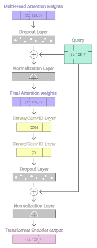
Transformer Encoder Layer

The single- and multi-head attention mechanisms (self-attention) are now aggregated into a transformer encoder layer. Each encoder layer incorporates a self-attention sublayer and a feedforward sublayer. The feedforward sublayer consists of two dense layers with ReLU activation in between.

On a side note, the dense layers can be replaced with 1-dimensional convolutional layers if the Conv-layers have a kernel size and stride of 1. The math of a dense layer and a convolutional layer with the described configuration is the same.

Each sublayer is followed by a dropout layer, after the dropout, a residual connection is formed by adding the initial Query input to both sublayer outputs. Concluding each sublayer a normalization layer placed after the residual connection addition to stabilize and accelerate the training process.

Now we have a ready to use Transformer layer, which can be easily stacked to improve a model’s performance. Since we do not need any Transformer decoder layers our implemented Transformer architecture is very similar to the BERT [2] architecture. Although, the differences are the time embeddings and our transformer can handle a 3-dimensional time-series instead of a simple 2-dimensional sequence.

If you want to dive into the code instead, here we go.

Model architecture with Time Embeddings and Transformer layers

In conclusion, we first initialize the time embedding layer as well as 3 Transformer encoder layers. After the initialization, we stack a regression head onto the last transformer layer and the training process begins.

Results

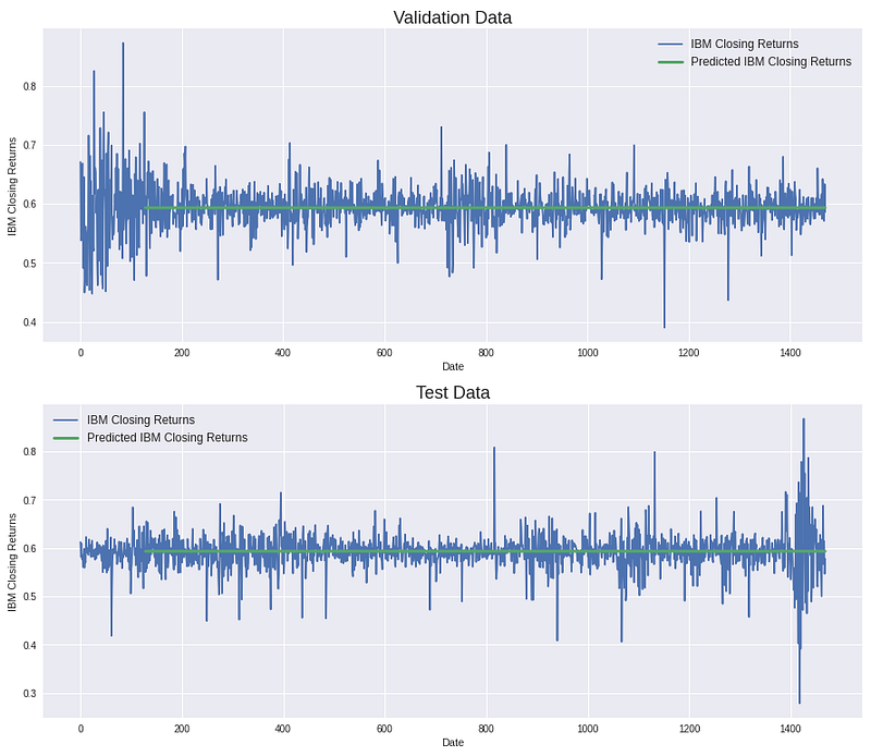
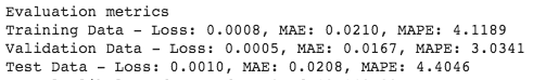
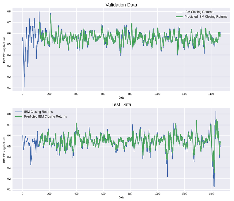
The training process has a total number of 35 epochs. After the training, we can see that our transform model is just predicting a flat line that is centered in between the daily stock price changes. When only using the IBM stock history even a transformer model is merely capable of predicting the linear trend of a stock’s development. Concluding that the historical price and volume data of a stock does only contain enough explanatory value for a linear trend prediction. However, when upscaling the dataset to thousands of stock tickers (1 Terabyte dataset) the results, look quite different 🙂.

Applying moving average to stock data — Feature engineering

As shown above, even the most advanced model architectures are not able to extract non-linear stock predictions from historical stock prices and volumes. However, when applying a simple moving average smoothing effect on the data (window size=10), the model is able to provide significantly better predictions (green line). Instead of predicting the linear trend of the IBM stock, the model is able to predict the up and downs, too. However, when observing carefully you can still see that the model has a large prediction delta on days with extreme daily change rate, hence we can conclude that we still have issues with outliers.

The disadvantage of applying a moving average effect is that the new dataset is not reflecting our original data anymore. Hence the predictions with the moving average effect cannot be used as input for our trading bot.

The performance increases due to the smoothing of the moving average effect can be achieved however without applying a moving average though. My latest research has shown that when extending the dataset to a large magnitude of stocks the same performance can be obtained.

All the code that has been presented in this article is part of a notebook that can be run end-to-end. The notebook can be found on GitHub.

Note from Towards Data Science’s editors: While we allow independent authors to publish articles in accordance with our rules and guidelines, we do not endorse each author’s contribution. You should not rely on an author’s works without seeking professional advice. See our Reader Terms for details.

Thank you,

Jan

Edited 1st June 2022:

In the past I’ve received a tone of feedback and requests to make my financial asset prediction models available and easily usable. It would help people to answer questions such as:

What are good assets to invest in? What do I put into my financial portfolio?

Let me introduce you to PinkLion www.pinklion.xyz

PinkLion is a product that lives on top of my code base to make daily asset data available for thousands of stocks, funds/ETFs, and crypto currencies. In addition, it allows asset analytics and portfolio optimisation on the fly by providing access to underlying prediction models.

At the moment the number of signups is still limited due to the massive amount of server resources needed for the individual calculations.

Feel free to give it a try and provide feedback. (It is still in a rough state) www.pinklion.xyz

Disclaimer

None of the content presented in this article constitutes a recommendation that any particular security, portfolio of securities, transaction, or investment strategy is suitable for any specific person. Futures, stocks, and options trading involves substantial risk of loss and is not suitable for every investor. The valuation of futures, stocks, and options may fluctuate, and, as a result, clients may lose more than their original investment.

References

[1] Why Self-Attention? A Targeted Evaluation of Neural Machine Translation Architectures https://arxiv.org/abs/1808.08946

[2] BERT: Pre-training of Deep Bidirectional Transformers for Language Understanding https://arxiv.org/abs/1810.04805

[3] Time2Vec: Learning a Vector Representation of Time https://arxiv.org/abs/1907.05321

[4] Attention Is All You Need https://arxiv.org/abs/1706.03762