Stock Market Trend Analysis With Hidden Memory Model & Long Short Term Memory

Today I am going to show you, how you can do stock market trend analysis with HMM and LSTM.

We are going to code a research paper, which is published online, check it here.

Structure of our code base:

.
├── .gitignore
├── FIGURE
│   ├── best_iter.png
│   ├── test1.jpg
│   ├── test2.jpg
│   ├── train1.jpg
│   └── train2.jpg
├── LICENSE
├── PAPER
│   └── 2104.09700.pdf
├── README.md
├── XGB_HMM
│   ├── GMM_HMM.py
│   ├── __pycache__
│   │   ├── GMM_HMM.cpython-36.pyc
│   │   ├── evaluate_A_pi.cpython-36.pyc
│   │   ├── form_B_matrix_by_XGB.cpython-36.pyc
│   │   ├── plot_result.cpython-36.pyc
│   │   ├── predict.cpython-36.pyc
│   │   ├── re_estimate.cpython-36.pyc
│   │   └── xgb.cpython-36.pyc
│   ├── form_B_matrix_by_XGB.py
│   ├── plot_result.py
│   ├── predict.py
│   ├── re_estimate.py
│   └── xgb.py
├── dataset_code
│   ├── HMM_duoyinzi.py
│   ├── HMM_hangqing.py
│   ├── __pycache__
│   │   ├── HMM_duoyinzi.cpython-36.pyc
│   │   ├── HMM_hangqing.cpython-36.pyc
│   │   ├── combine.cpython-36.pyc
│   │   ├── pred_proba_GMM.cpython-36.pyc
│   │   ├── pred_proba_XGB.cpython-36.pyc
│   │   └── process_on_raw_data.cpython-36.pyc
│   ├── combine.py
│   ├── form_df_all.py
│   ├── pred_proba_GMM.py
│   ├── pred_proba_XGB.py
│   └── process_on_raw_data.py
├── extracted_content.ipynb
├── extracted_content_5Humane.ipynb
├── extracted_content_5Humane_modified.ipynb
├── extracted_content_modified.ipynb
├── main_single_score.py
├── main_train_model.py
├── public_tool
│   ├── __pycache__
│   │   ├── bagging_balance_weight.cpython-36.pyc
│   │   ├── combine_allow_flag.cpython-36.pyc
│   │   ├── evaluate_plot.cpython-36.pyc
│   │   ├── form_accuracy.cpython-36.pyc
│   │   ├── form_index.cpython-36.pyc
│   │   ├── form_model_dataset.cpython-36.pyc
│   │   ├── random_cut.cpython-36.pyc
│   │   └── solve_on_outlier.cpython-36.pyc
│   ├── bagging_balance_weight.py
│   ├── combine_allow_flag.py
│   ├── evaluate_plot.py
│   ├── form_accuracy.py
│   ├── form_index.py
│   ├── form_model_dataset.py
│   ├── random_cut.py
│   └── solve_on_outlier.py
├── test.ipynb
└── train_model
    ├── GMM_HMM.py
    ├── LSTM.py
    ├── XGB_HMM.py
    ├── __pycache__
    │   ├── GMM_HMM.cpython-36.pyc
    │   ├── LSTM.cpython-36.pyc
    │   ├── XGB_HMM.cpython-36.pyc
    │   ├── train_HMM_model.cpython-36.pyc
    │   └── train_LSTM_model.cpython-36.pyc
    ├── train_HMM_model.py
    └── train_LSTM_model.py

Now let’s start coding:

import pickle
import numpy as np
from dataset_code.process_on_raw_data import form_raw_dataset, df_col_quchong
from dataset_code.HMM_duoyinzi import solve2, form_model_dataset, form_model
from public_tool.evaluate_plot import evaluate_plot
import warnings
warnings.filterwarnings("ignore")

if __name__ == '__main__':
    
    temp = pickle.load(open('save/classified by id/000001.XSHE.pkl', 'rb'))
    temp = df_col_quchong(temp)
    temp = [i for i in temp.columns]
    feature_list = temp[temp.index('AccountsPayablesTDays'):]
    score_record = np.zeros(len(feature_list))

    for i in range(len(feature_list)):

        now_feature = [feature_list[i]]

        dataset, label, lengths, col_nan_record = form_raw_dataset(now_feature, label_length=3, verbose=False)

        if len(label) == 0:
            print('skip ' + now_feature[0])
            continue

        solved_dataset, allow_flag = solve2(dataset, now_feature, now_feature)

        train_X, train_label, train_lengths = form_model_dataset(solved_dataset, label, allow_flag, lengths)

        model = form_model(train_X, train_lengths, 3, 'diag', 1000, verbose=False)

        score = evaluate_plot(model, train_X, train_label, train_lengths)
        score_record[i] = score

        print('all:%s, now:%s, ' % (len(feature_list), i + 1) + now_feature[0] + ': score:%s' % score)

        pickle.dump([score_record, feature_list], open('save/duoyinzi_solve2_score.pkl', 'wb'))

    pickle.dump([score_record, feature_list], open('save/duoyinzi_solve2_score.pkl', 'wb'))

The Python code is involved with loading, processing, and evaluating dataset features using machine learning models, specifically Hidden Markov Models HMMs. It uses libraries such as pickle, numpy, and various custom modules from a package called dataset_code and a module public_tool. Initially, the script disables warnings to keep the output clean. The main process begins by loading a dataset from a pickle file. It assumes that the data has some form of structure, as it proceeds to apply a deduplication function, df_col_quchong, to the DataFrames columns.

Next, the code extracts a list of features starting from a specific feature named AccountsPayablesTDays until the end of the list. It then initializes a score record array to keep track of the evaluation scores of the features. In a loop over all the features, the code prepares a raw dataset for each feature with certain parameters, filtering out any features without labels. Each feature is subjected to a process using an HMM, solve2, to classify data points and then used to create a training dataset. A model is formed using the training dataset and specific parameters for the HMM.

Each model is evaluated using the evaluate_plot function, which presumably assesses the models performance and returns a score. The score for each features model is stored in the score record array. Finally, the scores and the features list are saved into a pickle file for later use. This record-keeping ensures that the evaluation scores can be reviewed or utilized in subsequent analysis without re-running the entire process.

The overall purpose of this code is to process a dataset through deduplication, feature extraction, training via Hidden Markov Models, and scoring the performance of these models on a feature-by-feature basis for further analysis.

Main Train Model

from train_model.train_HMM_model import train_HMM_model
from train_model.train_LSTM_model import train_LSTM_model

if __name__ == '__main__':

    n_states = 3
    train_HMM_model(n_states)

    train_LSTM_model()

The Python script is designed to train two different types of statistical models using separate modules imported from a package called train_model.

The scripts purpose is to execute the training process for a Hidden Markov Model HMM and a Long Short-Term Memory LSTM neural network when it is run as the main code. When the script is executed, the if __name__ == __main__: block ensures that the model training functions are called only if this script is being run directly not when imported as a module in another script. Inside this block, the script first sets the variable n_states to 3, which is likely the number of hidden states desired for the HMM.

The function train_HMM_modeln_states is then called, importing from the train_HMM_model file inside the train_model package. This function takes the number of hidden states as an argument and proceeds to train the HMM with that configuration. After the HMM training, the script calls the function train_LSTM_model with no arguments, signifying that this function may have its parameters set inside the function or use a predefined configuration.

This function comes from the train_LSTM_model file within the train_model package and is responsible for training an LSTM model, a type of recurrent neural network known for its ability to remember long-term dependencies.

import sys
import numpy as np
from public_tool.form_index import form_index


def combine(X1, X2, allow_flag1, allow_flag2, label, lengths):

    if not (type(X1) == type(allow_flag1) or type(X2) == type(allow_flag2)):
        sys.exit('x 和 allow_flag的输入格式不一致')

    list_flag1 = type(X1) == list
    list_flag2 = type(X2) == list

    X = np.zeros((len(label), 0))
    allow_flag = np.zeros(len(label))
    count = 0

    if list_flag1 == 1:
        for i in range(len(X1)):
            X = np.column_stack(X, X1[i])
            allow_flag += allow_flag1[i]
            count += 1
    else:
        X = np.column_stack((X, X1))
        allow_flag += allow_flag1
        count += 1
    if list_flag2 == 1:
        for i in range(len(X2)):
            X = np.column_stack((X, X2[i]))
            allow_flag += allow_flag2[i]
            count += 1
    else:
        X = np.column_stack((X, X2))
        allow_flag += allow_flag2
        count += 1
    allow_flag[allow_flag < count] = 0
    allow_flag[allow_flag == count] = 1

    result_X = np.zeros((0, X.shape[1]))
    result_label = np.zeros(0)
    result_lengths = []

    for i in range(len(lengths)):
        begin_index, end_index = form_index(lengths, i)

        now_X = X[begin_index:end_index]
        now_allow_flag = allow_flag[begin_index:end_index]
        now_label = label[begin_index:end_index]

        temp = np.logical_and(now_allow_flag == 1, now_label != -2)

        result_X = np.row_stack((result_X, now_X[temp]))
        result_label = np.hstack((result_label, now_label[temp]))
        result_lengths.append(sum(temp))

    return result_X, result_label, result_lengths

This Python code defines a function, combine, that is intended to combine data from two sources and provide a filtered result based on some conditions. The function takes six parameters: two inputs X1 and X2, which can either be lists or arrays; two corresponding allow flags allow_flag1 and allow_flag2, which are used to indicate which elements of the inputs are permitted; a label array that categorizes input data; and lengths, which seems to define segment lengths within the combined data.

The function initially checks if X1 and X2 match in type with their corresponding allow flags. If not, the code exits with an error message. If their types are consistent, the function proceeds. The function then initializes an empty array X and an allow_flag array with zeros, both of which are intended to be filled with combined data from X1 and X2. It determines whether the input data comes in list format, and accordingly loops through the lists to stack the data horizontally in the X matrix and accumulates the corresponding allow flags. If the inputs are not lists, it performs similar operations without looping.

The accumulated allow_flag array is then processed to create a filter, setting the flag to zero where the element count is less than the number of inputs combined and to one where the count is equal to the number of inputs. Next, the function creates an empty matrix, result_X and an array, result_label, along with an empty list result_lengths. It then loops through the entries specified by lengths to slice X and allow_flag into segments, and uses logical conditions to filter these segments based on the allow flag and label conditions excluding elements labeled as -2. It combines these filtered segments into result_X and result_label, respectively, and computes the lengths of these segments to populate result_lengths.

Finally, combine returns three processed and filtered results: result_X, result_label, and result_lengths, which contain the combined data satisfying the specified conditions, the corresponding filtered labels, and the lengths of the filtered segments, respectively.

import os
import pandas as pd
import numpy as np 
import pickle


file_path = 'C:/Users/Administrator/Desktop/program/data/hangqing/'
file_list = os.listdir(file_path)
columns_name = pd.read_csv(file_path+file_list[0]).columns

hangqing_record = []
temp_record = pd.DataFrame(columns=columns_name)
for i in range(len(file_list)):
    now_path = file_path+file_list[i]
    now_df = pd.read_table(now_path, sep=',')
    temp_record = pd.concat((temp_record, now_df), axis=0)
    if (i+1) % 50 == 0 or (i+1) == len(file_list):
        del temp_record['Unnamed: 0']
        del temp_record['Unnamed: 25']
        hangqing_record.append(temp_record)
        temp_record = pd.DataFrame(columns=columns_name)
    print('all:%s, now:%s' % (len(file_list), i+1))

for i in range(len(hangqing_record)):
    if i == 0:
        hangqing_df = hangqing_record[0]
    else:
        hangqing_df = pd.concat((hangqing_df, hangqing_record[i]), axis=0)
del hangqing_record


file_path = 'C:/Users/Administrator/Desktop/program/data/duoyinzi/'
file_list = os.listdir(file_path)
columns_name = pd.read_csv(file_path+file_list[0]).columns

duoyinzi_record = []
temp_record = pd.DataFrame(columns=columns_name)
for i in range(len(file_list)):
    now_file = file_list[i]
    now_path = file_path+now_file
    tradeDate = now_file[0:4]+'-'+now_file[4:6]+'-'+now_file[6:8]
    now_df = pd.read_table(now_path, sep=',')
    now_df['tradeDate'] = tradeDate
    temp_record = pd.concat((temp_record, now_df), axis=0)
    if (i+1) % 30 == 0 or (i+1) == len(file_list):
        del temp_record['Unnamed: 0']
        del temp_record['Unnamed: 248']
        duoyinzi_record.append(temp_record)
        temp_record = pd.DataFrame(columns=columns_name)
    print('all:%s, now:%s' % (len(file_list), i+1))



unique_id = np.unique(hangqing_df['secID'].values)

duoyinzi_columns = duoyinzi_record[0].columns
for i in range(len(unique_id)):
    now_id = unique_id[i]
    now_hangqing_df = hangqing_df[hangqing_df['secID'] == now_id]
    now_duoyinzi_df = pd.DataFrame(columns=duoyinzi_columns)
    for temp in duoyinzi_record:
        now_temp = temp[temp['secID'] == now_id]
        if now_temp.shape[0] != 0:
            now_duoyinzi_df = pd.concat((now_duoyinzi_df, now_temp), axis=0)
    now_df = pd.merge(now_hangqing_df, now_duoyinzi_df, on=['secID', 'tradeDate'], how='left')
    pickle.dump(now_df, open('save/classified by id/'+now_id+'.pkl', 'wb'))
    print('all:%s, now:%s' % (len(unique_id), i+1))

The purpose of the code is to aggregate and merge different sets of data from CSV files likely stock market data and organize them by security identifiers into serialized pickle files. The code begins by defining a file path where the CSV files are located and loading the list of file names in that directory. It then reads the column names from the first file to use as a template for creating dataframes. It iterates over each file, reads the contents, and appends them to a temporary dataframe.

After every 50 files or the end of the list, it removes two unnamed columns and adds the cleaned dataframe to a list. It then prints progress updates. After processing all files in the first directory, the script concatenates the collected dataframes into one large dataframe. It then repeats a similar process for a different directory of CSV files, representing a different set of market data, possibly option or derivatives data named duoyinzi. This time, it modifies each dataframe to include a tradeDate derived from the filename and performs concatenation every 30 files or at the end of the list.

Once both sets of data are processed, the script extracts unique security identifiers secID from the first set of data. It then loops through each unique identifier, filters the corresponding rows in both sets of dataframes, and merges them based on the secID and tradeDate. Each combined dataframe is then serialized and saved as a pickle file, named after the unique security identifier. Lastly, the script prints out progress messages as it loops through each unique identifier, providing feedback on the number of completed tasks versus the total number of unique identifiers to process.

LSTM


import numpy as np
from keras.models import Sequential
from keras.layers import Dense, LSTM, Dropout
from keras.layers.advanced_activations import LeakyReLU
from sklearn.preprocessing import MinMaxScaler
from keras.callbacks import EarlyStopping
from sklearn.preprocessing import LabelBinarizer
from public_tool.bagging_balance_weight import bagging_balance_weight
from keras.layers import BatchNormalization
from keras.optimizers import SGD
from public_tool.form_index import form_index
from public_tool.random_cut import random_cut
from public_tool.form_accuracy import form_accuracy
from keras.models import load_model
import pickle


def form_LSTM_dataset(X, y, lengths, T):
    result_X = []
    result_y = []
    for i in range(len(lengths)):
        begin_index, end_index = form_index(lengths, i)
        now_X = X[begin_index:end_index]
        now_y = y[begin_index:end_index]

        for j in range(len(now_y) - T):
            result_X.append(now_X[j:j + T])
            result_y.append(now_y[j + T])

    result_X = np.array(result_X)

    return result_X, result_y


def self_LSTM(X, y, lengths, file_name):    
    mms = MinMaxScaler()
    X = mms.fit_transform(X)

    T = 10
    X_LSTM, y_LSTM = form_LSTM_dataset(X, y, lengths, T)

    
    lb = LabelBinarizer()
    y_LSTM = lb.fit_transform(y_LSTM)

    
    X_train, y_train, X_valid, y_valid = random_cut(X_LSTM, y_LSTM, 5)
    X_train, y_train = bagging_balance_weight(X_train, y_train)

    
    model = Sequential()

    model.add(Dropout(0.2))
    model.add(LSTM(40))
    model.add(BatchNormalization())
    model.add(LeakyReLU(alpha=0.02))

    model.add(Dropout(0.2))
    model.add(Dense(30, kernel_initializer='glorot_normal'))
    model.add(BatchNormalization())
    model.add(LeakyReLU(alpha=0.02))

    model.add(Dropout(0.2))
    model.add(Dense(3, activation='softmax'))

    sgd = SGD(lr=0.01, decay=1e-4, momentum=0.9, nesterov=True)
    model.compile(loss='categorical_crossentropy', optimizer=sgd, metrics=['accuracy'])

    
    model.fit(X_train,
              y_train,
              batch_size=int(X_train.shape[0] / 5),
              epochs=10000,
              verbose=2,
              validation_split=0.0,
              validation_data=(X_valid, y_valid),
              shuffle=True,
              class_weight=None,
              sample_weight=None,
              initial_epoch=0,
              callbacks=[])

    print('train    ', form_accuracy(X_train, y_train, model))
    print('valid   ', form_accuracy(X_valid, y_valid, model))

    mms_file_name = 'C:/Users/Administrator/Desktop/HMM_program/save' + file_name + '_mms.pkl'
    pickle.dump(mms, open(mms_file_name, 'wb'))
    model_file_name = 'C:/Users/Administrator/Desktop/HMM_program/save' + file_name + '_model.h5'
    model.save(model_file_name)

The Python code describes the process of training a deep learning model, specifically a Long Short-Term Memory LSTM network, for some classification task. The code makes use of Keras, a high-level neural network API, which runs on top of TensorFlow or Theano.

First, the code imports necessary libraries for numerical operations, machine learning model building, preprocessing, and utility functions which seem to be custom functions not included in standard libraries. The form_LSTM_dataset function appears to take in a set of features X, a set of labels y, a list of sequence lengths, and a window size T, and transforms the data into a format suitable for training an LSTM network. This involves segmenting the input data into subsequences of length T.

The main function self_LSTM preprocesses the input features using MinMaxScaler to normalize the data. It then uses the form_LSTM_dataset function to convert the data into the LSTM format. The labels are binarized using LabelBinarizer, implying a classification task. The data is then split into training and validation sets via a custom function random_cut, and training data is balanced using bagging_balance_weight. The code then defines the LSTM network model with several layers, including dropout layers to prevent overfitting, batch normalization layers for faster convergence, and dense layers for prediction. It uses a LeakyReLU activation function for the hidden layers and a softmax activation for the output layer to handle the classification.

The model is compiled with the Stochastic Gradient Descent SGD optimizer to minimize the categorical cross entropy loss function, a common choice for multi-class classification tasks. The model is trained using the training data with a specified batch size and number of epochs, without using any early stopping or other callbacks. After training, the accuracy of the model is assessed on both the training and validation datasets with a custom form_accuracy function.

Finally, the MinMaxScaler and the trained LSTM model are saved to the disk at specified locations with file names incorporating an external variable file_name, indicating that the model and its scaler can be reloaded for later use or analysis.

Train LSTM Model

from dataset_code.process_on_raw_data import form_raw_dataset
import pickle
from dataset_code import HMM_duoyinzi, HMM_hangqing
from dataset_code.pred_proba_GMM import pred_proba_GMM
from dataset_code.combine import combine
from dataset_code.pred_proba_XGB import pred_proba_XGB
from train_model.LSTM import self_LSTM


def train_LSTM_model():
    feature_col_hangqing = ['preClosePrice', 'openPrice', 'closePrice', 'turnoverVol', 'highestPrice', 'lowestPrice']
    score, feature_name = HMM_duoyinzi.load_duoyinzi_single_score()
    feature_col_duoyinzi = HMM_duoyinzi.type_filter(score, feature_name, 0.1)
    feature_col = feature_col_hangqing
    _ = [[feature_col.append(j) for j in i] for i in feature_col_duoyinzi]
    dataset, label, lengths, col_nan_record = form_raw_dataset(feature_col, 5)

    
    
    solved_dataset1, allow_flag1 = HMM_hangqing.solve_on_raw_data(dataset, lengths, feature_col)
    model = pickle.load(open('C:/Users/Administrator/Desktop/HMM_program/save/hangqing_GMM_HMM_model.pkl', 'rb'))
    pred_proba1 = pred_proba_GMM(model, solved_dataset1, allow_flag1, lengths)

    
    pred_proba2 = []
    allow_flag2 = []
    model = pickle.load(open('C:/Users/Administrator/Desktop/HMM_program/save/duoyinzi_GMM_HMM_model.pkl', 'rb'))
    for i in range(len(feature_col_duoyinzi)):
        temp_solved_dataset, temp_allow_flag = HMM_duoyinzi.solve_on_raw_data(dataset, lengths, feature_col, feature_col_duoyinzi[i])
        temp_model = model[i]
        temp_pred_proba = pred_proba_GMM(temp_model, temp_solved_dataset, temp_allow_flag, lengths)
        pred_proba2.append(temp_pred_proba)
        allow_flag2.append(temp_allow_flag)

    
    final_X, final_y, final_lengths = combine(pred_proba1, pred_proba2, allow_flag1, allow_flag2, label, lengths)

    
    self_LSTM(final_X, final_y, final_lengths, 'GMM_HMM_LSTM')

    
    
    solved_dataset1, allow_flag1 = HMM_hangqing.solve_on_raw_data(dataset, lengths, feature_col)
    temp = pickle.load(open('C:/Users/Administrator/Desktop/HMM_program/save/hangqing_XGB_HMM_model.pkl', 'rb'))
    A, model, pi = temp[0], temp[1], temp[2]
    pred_proba1 = pred_proba_XGB(A, model, pi, solved_dataset1, allow_flag1, lengths)

    
    pred_proba2 = []
    allow_flag2 = []
    model = pickle.load(open('C:/Users/Administrator/Desktop/HMM_program/save/duoyinzi_XGB_HMM_model.pkl', 'rb'))
    for i in range(len(feature_col_duoyinzi)):
        temp_solved_dataset, temp_allow_flag = HMM_duoyinzi.solve_on_raw_data(dataset, lengths, feature_col, feature_col_duoyinzi[i])
        temp_A, temp_model, temp_pi = model[i][0], model[i][1], model[i][2]
        temp_pred_proba = pred_proba_XGB(temp_A, temp_model, temp_pi, temp_solved_dataset, temp_allow_flag, lengths)
        pred_proba2.append(temp_pred_proba)
        allow_flag2.append(temp_allow_flag)

    
    final_X, final_y, final_lengths = combine(pred_proba1, pred_proba2, allow_flag1, allow_flag2, label, lengths)

    
    self_LSTM(final_X, final_y, final_lengths, 'XGB_HMM_LSTM')

This Python code is designed for training machine learning models in finance, particularly for market prediction or analysis. It is composed of several parts that import necessary functions, handle data preprocessing, feature extraction, and model training.

Initially, the code imports a series of modules and functions that will be used for data processing and model predictions, such as HMM Hidden Markov Model functions for processing different features, GMM Gaussian Mixture Model for probabilistic predictions, a combination module, and XGB eXtreme Gradient Boosting for boosted tree predictions. These utilities are likely part of a custom library named dataset_code, and an LSTM Long Short-Term Memory neural network module is imported from a train_model package.

The purpose of the code is to train two different versions of an LSTM model — one with features processed by a GMM-HMM algorithm and the other with features processed by an XGB-HMM algorithm. The code operates in the following manner:

It starts by defining a range of financial features that pertain to stock market prices and volumes termed as feature_col_hangqing.
It then loads and filters additional features, potentially from a linguistic or textual analysis duoyinzi, according to their scores.
A raw dataset is formed from the specified features with the function form_raw_dataset, and this dataset undergoes preprocessing through HMM algorithms HMM_hangqing and HMM_duoyinzi.
Pre-trained GMM-HMM models for each feature set are loaded using the pickle library, and the probability predictions pred_proba are generated for each dataset.
These predictions are combined along with their corresponding flags which might indicate usable vs. non-usable predictions using the combine function to form training sets for the LSTM models final_X, final_y, final_lengths.
An LSTM model is trained with the GMM-HMM processed features using the self_LSTM function and then saved with a specific name indicating its a GMM_HMM_LSTM model.
A similar process is repeated, except in place of GMM-HMM models, XGB-HMM models are loaded and used for generating predictions.
Finally, another LSTM model is trained with these new predictions and called the XGB_HMM_LSTM model.

The overall aim of this code is to experiment with two different sets of features and see which combination after being processed by HMM and predicted by GMM/XGB produces better results when used to train an LSTM model for financial time series prediction. The code handles much of the data processing, model loading, prediction generation, and LSTM model training autonomously, implying that this could be part of a larger automated trading system or forecasting tool.

Prediction

import numpy as np
from public_tool.form_index import form_index


def self_pred(B, lengths, A, pi):
    log_likelihood_list = []
    n_states = len(pi)
    init_flag = 1

    for i in range(len(lengths)):
        begin_index, end_index = form_index(lengths, i)
        now_B = B[begin_index:end_index].copy()
        now_state = np.zeros(lengths[i])
        now_state_proba = np.zeros((lengths[i], n_states))

        for j in range(lengths[i]):

            if j == 0:
                now_state_proba[j] = now_B[j] * pi
            else:
                for k in range(n_states):
                    temp = now_state_proba[j-1] * A[:, k] * now_B[j, k]
                    now_state_proba[j, k] = max(temp)
            now_state_proba[j] = now_state_proba[j] / np.sum(now_state_proba[j])
            now_state[j] = np.argmax(now_state_proba[j])

        for j in range(lengths[i]):
            if j == 0:
                now_log_likelihood = np.log(pi[int(now_state[j])]) + np.log(now_B[j, int(now_state[j])])
            else:
                now_log_likelihood += np.log(A[int(now_state[j-1]), int(now_state[j])]) + np.log(now_B[j, int(now_state[j])])

        if init_flag == 1:
            state = now_state
            state_proba = now_state_proba
            init_flag = 0
        else:
            state = np.hstack((state, now_state))
            state_proba = np.row_stack((state_proba, now_state_proba))

        log_likelihood_list.append(now_log_likelihood)

    log_likelihood = 0
    for i in log_likelihood_list:
        log_likelihood += i

    return state, state_proba, log_likelihood

The Python code defines a function named self_pred that takes in four arguments: B, lengths, A, and pi. This function seems to be implementing a sequence prediction algorithm using a Hidden Markov Model HMM or a similar probabilistic model where states are hidden and only the outputs emissions are observed.

The purpose of the code is to predict the most likely sequence of hidden states for given observed sequences B based on the model parameters A and pi. The lengths argument is a list of integers indicating the lengths of different observed sequences within B. The function uses logarithms of probabilities log_likelihood to avoid numerical underflow, which can occur when working with very small probabilities.

Firstly, the function initializes some variables to store the predicted states, their probabilities, and the log likelihood of the sequences given the model. It then iterates over each observed sequence which is segmented based on the lengths provided. For each segment, the function duplicates the corresponding part of B and initializes the state probability matrix and the state sequence. Inside the main loop, it uses dynamic code to compute the most likely state at each time step now_state and its probability now_state_proba, given the observations.

The model parameters A state transition probabilities and pi initial state probabilities are used to calculate these probabilities. The resulting likelihood of the sequence given the model is accumulated in log_likelihood_list. After iterating through all the segments, the code concatenates the predicted states and their probabilities to form the final output. It then sums the log likelihood of all the individual sequences to get the overall log likelihood of the observed sequences given the model.

Finally, the function returns a tuple containing the concatenated predicted states state, the row-wise stacked state probabilities state_proba, and the total log likelihood log_likelihood of the observations given the model.

Plotting Results

import matplotlib.pyplot as plt
import numpy as np


def form_color_dict(S, label):
    
    n_states = len(np.unique(S))
    count = np.zeros(n_states)
    record = np.zeros((n_states, 3))

    S = np.delete(S, np.where(label == -2), 0)
    label = np.delete(label, np.where(label == -2), 0)

    for i in range(len(S)):
        temp = int(S[i])
        count[temp] += 1
        record[temp, int(label[i])+1] += 1

    for i in range(n_states):
        record[i] = record[i]/count[i]

    blue_index = np.argmax(record[:, 1])

    else_index = [0, 1, 2]
    else_index.remove(int(blue_index))

    index1 = else_index[0]
    index2 = else_index[1]
    flag1 = record[index1, 2] - record[index1, 0]
    flag2 = record[index2, 2] - record[index2, 0]
    if np.abs(flag1) > np.abs(flag2):
        if flag1 > 0:
            red_index = index1
            green_index = index2
        else:
            green_index = index1
            red_index = index2
    else:
        if flag2 > 0:
            red_index = index2
            green_index = index1
        else:
            green_index = index2
            red_index = index1

    print(record)

    true = dict(zip([green_index, red_index, blue_index], ['g', 'r', 'b']))

    return true


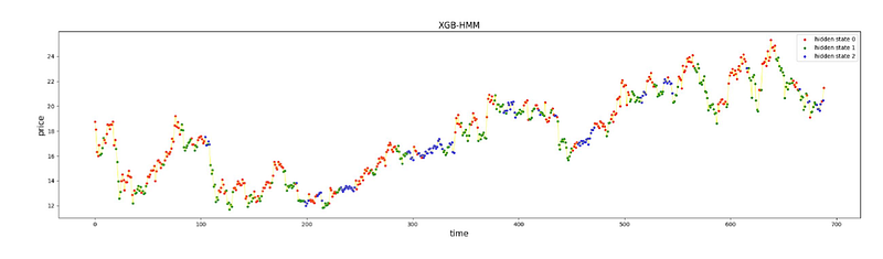
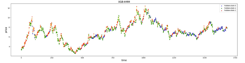
def plot_result(price, label, S, new_S, n_states, record_log_likelihood, record_plot_score):
    plt.figure(1, figsize=(100, 50))
    show_x = np.array([i for i in range(len(S))])

    plt.subplot(212)
    plt.title('XGB-HMM', size=15)
    plt.ylabel('price', size=15)
    plt.xlabel('time', size=15)
    _ = form_color_dict(S, label)
    true = form_color_dict(new_S, label)

    for i in range(n_states):
        color = true[i]
        temp = (new_S == i)
        plt.scatter(show_x[temp], price[temp], label='hidden state %d' % i, marker='o', s=10, c=color)
        plt.legend(loc='upper right')
    plt.plot(price, c='yellow', linewidth=0.5)

    plt.subplot(211)
    plt.title('GMM-HMM', size=15)
    plt.ylabel('price', size=15)
    plt.xlabel('time', size=15)

    for i in range(n_states):
        color = true[i]
        temp = (S == i)
        plt.scatter(show_x[temp], price[temp], label='hidden state %d' % i, marker='o', s=10, c=color)
        plt.legend(loc='upper right')
    plt.plot(price, c='yellow', linewidth=0.5)

    
    fig = plt.figure(2, (400, 400))
    ax1 = fig.add_subplot(111)
    ax1.plot(np.array([np.nan] + record_log_likelihood), label='log likelihood', c='r')
    ax1.set_ylabel('log likelihood', size=20)
    ax1.set_xlabel('iteration', size=20)
    plt.legend(loc='upper left')

    ax2 = ax1.twinx()
    ax2.plot(np.array(record_plot_score), label='plot score', c='b')
    ax2.set_ylabel('plot score', size=20)

    plt.legend(loc='upper right')

    index = np.argmax(np.array(record_log_likelihood))
    ax1.scatter(np.array(index+1), np.array(record_log_likelihood[index]), marker='o', c='k', s=60)
    ax1.annotate('best iteration', size=20, xy=(index+1, record_log_likelihood[index]),
                 xytext=(index-5, record_log_likelihood[index]*1.05), arrowprops=dict(facecolor='black', shrink=1))

    plt.show()

    return true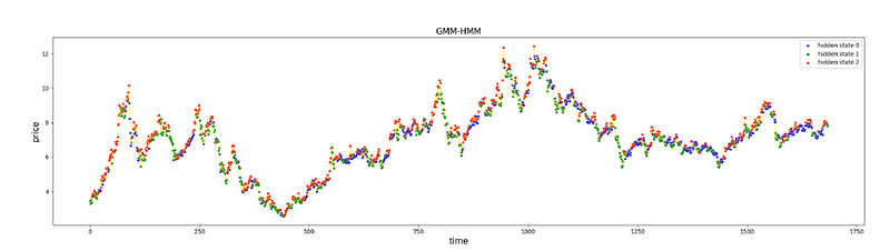

The Python code is designed to analyze and visualize the results of a statistical model applied to a times series data representing prices. The code is using two main libraries; matplotlib for plotting graphs and numpy for numerical computations.

The first function form_color_dict accepts arrays S and label. It processes these arrays to generate a dictionary that maps certain states to color labels g green, r red, and b blue, based on the content of S and label arrays. It filters out elements in both arrays marked with -2, computes the frequency of each unique state in S, and then labels states by comparing the occurrence of positive and negative values in label.

Finally, it prints the resulting record array and returns the color dictionary. The second function plot_result is used to plot the results of the model comparison between two approaches labeled as XGB-HMM and GMM-HMM. It utilizes several subplots to display different aspects of the data and the models performance. In two of the subplots, it plots the price over time, where data points are color-coded to represent the hidden state assigned to them by two different versions of the model.

The function then creates another plot showing the evolution of the log-likelihood and plot score over iterations, highlighting the best iteration. The purpose of the code is to interpret the results of a Hidden Markov Model HMM applied to pricing data likely stock prices or similar financial data, to reveal underlying hidden states in the data, and to compare the performance of two variants of the HMM XGB-HMM and GMM-HMM. It visualizes the segmentation of price data by hidden states and the improvement of model likelihood over time, providing insights into the models behavior and aiding in the identification of the best-performing iteration.

Download the source code from here: Visit This Link!