Step by Step Guides for EDA Process with Python’s Codes

What is EDA?

Exploratory data analysis (EDA) is a thorough investigation of the whole data sets mainly with visualization plots before conducting and building data mining models for the data scientists.

Why EDA is necessary for data mining project?

Performing EDA will reveal the main characteristics of data sets such as numbers of records, attributes, missing values and outliers, correlation between attributes, possible multicollinearity, necessity of dimension reduction, skewness of data, data’s distribution patterns, etc. Thus, EDA process is cleaning up the data set to get the valuable insights of the data we are working with.

EDA Steps with Python

• Loading the Data set

df = pd.read_csv('/Users/users/Desktop/stroke.csv')
df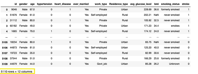

From this, it’s noted that there are 5110 rows and 12 columns.

• Finding out Data Types of Variables and Null Values

df.info()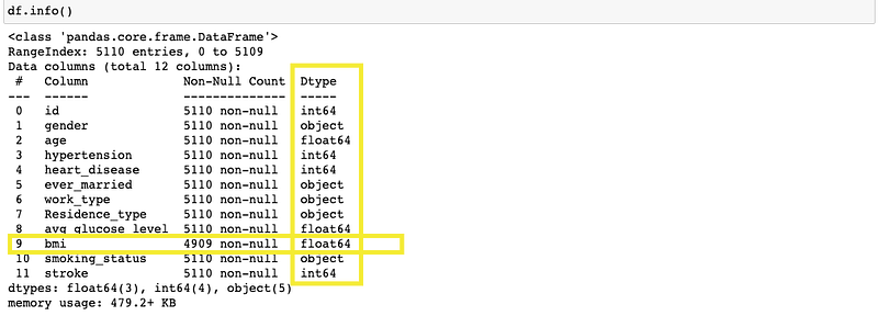 

df.info() will reveal the names of the variables and data types of each variables. It will also show the null values present in each variable. For example, there’s only 4909 record without null values in bmi variable. That tells us that 201 missing values in the bmi variable.

• Another Way To Finding Out Total Counts of Null Values

df.isna.sum()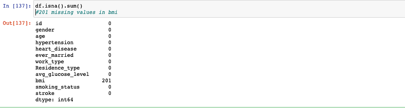

It’s a good strategy to replace the null values with mean instead of dropping them since it will retain the full records.

#replacing bmi na value with mean
df['bmi'] = df['bmi'].fillna((df['bmi'].mean()))

#Double checking null values again
df.isna.sum()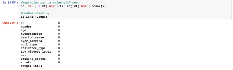

• Summary Statistics of whole data set

df.describe()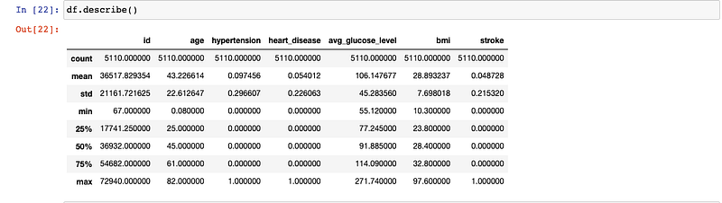

• Unique Variables

Let’s look at the unique counts from each variable. For example, we will expect to see 2 unique counts from heart_disease variable (Yes and No).

df.nunique()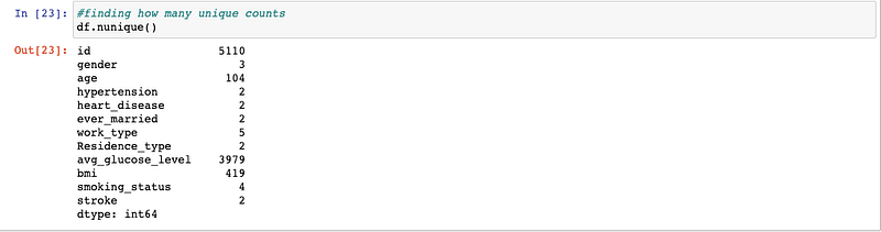

Visualizations

Visualization is an essential step in EDA process.

To get started, let’s assign the numerical variables under num_col so that we don’t need to list out the variables every single time.

num_col = df[['age','hypertension','heart_disease','avg_glucose_level','bmi']]
cat_col = df[['gender','ever_married','work_type','Residence_type','smoking_status']]

• Visualization of Numerical Variables

#visualizing numerical variables

plt.figure(figsize=(20, 12))

for i, column in enumerate(num_col,1):
    plt.subplot(3, 2, i)
    sns.distplot(x=df[column],color='blue') 
    plt.legend() 
    plt.xlabel(column)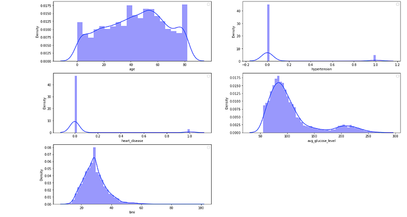

From these plots, all of the variables show the skewness and not normally distributed.

Let’s check the target variable (stroke) distribution

target= 'stroke'

df.hist(target, color='yellow')

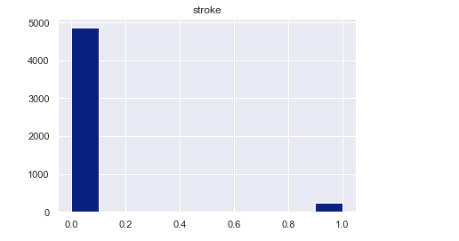
From the plot, class imbalance is observed between stroke (Yes=1 and No=0).

• Visualization for Correlation with Heatmap

corr = df.corr()
fig, ax = plt.subplots()
fig.set_size_inches(12,11)
sns.heatmap(corr, annot=True, cmap="Purples", center=0, ax=ax)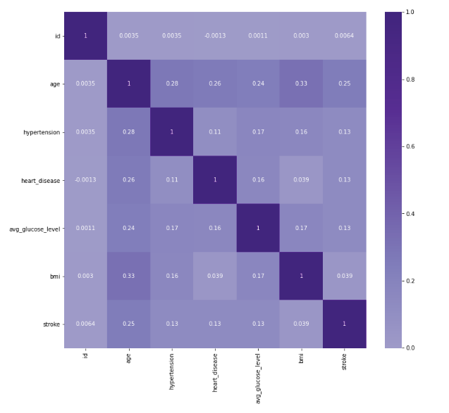

No strong correlation is observed among the attributes.

So these are the steps involved in EDA process. Another essential step of EDA process is finding out the outliers and removing them. We will talk about that in the next topic. Stay tuned!