
Step-by-Step Guide to Bayesian Optimization: A Python-based Approach
Building the Foundation: Implementing Bayesian Optimization in Python

Bayesian optimization is a technique used for the global (optimum) optimization of black-box functions.
A black box is a system whose internal workings are unknown to the observer. She can only have access to the inputs and outputs of the system but does not have knowledge of how the system arrives at outputs based on the inputs. In the context of optimization, a black box function refers to an objective function.
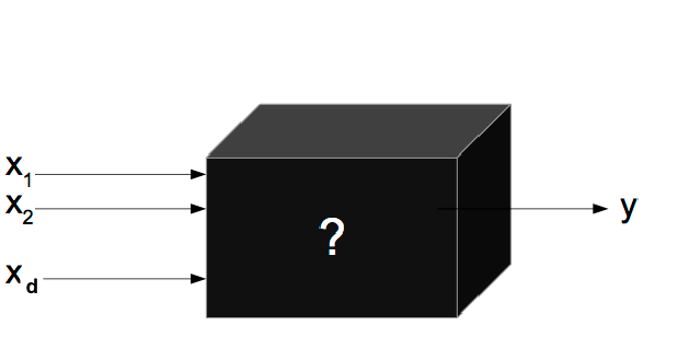
To illustrate, consider a function f that is inaccessible to us. We cannot directly access f or compute its gradients. Our only available information is providing an input x and receiving a noisy estimation (or without any noise) of the true output.
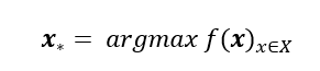
Our objective is to optimize the underlying value within the black box function f according to our purpose, maximizing it for example.
In traditional optimization methods, such as grid search or random search, the objective function is evaluated at a predefined set of points. However, these methods can be computationally expensive and inefficient when dealing with high-dimensional or noisy functions.

Bayesian optimization offers several advantages over traditional methods. Firstly, it efficiently handles expensive and noisy function evaluations by building a probabilistic surrogate model, which captures the uncertainty and guides the search process intelligently.
It incorporates prior knowledge or beliefs about the objective function, enabling more informed decision-making.
It also balances exploration and exploitation. Exploration allows for a broader exploration of the search space, potentially discovering better solutions, while exploitation focuses on exploiting the known promising areas to optimize the current best solution. Balancing these two aspects is crucial to finding better solutions and refining the best solution.

Classical bandit algorithms make use of frequentist bounds to model the unknown function. Bandit problems are a class of sequential decision-making problems that involve selecting actions from a set of options (arms) over a series of steps or time periods. Each arm has an unknown reward distribution associated with it, and the goal is to maximize the cumulative reward obtained by selecting the arms strategically.
In the depicted cube shape, there are three metrics represented along three axes, providing an understanding of the variations in mindsets at a broader level.

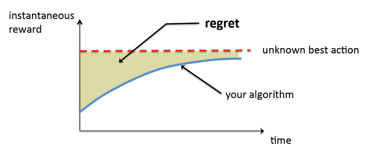
The performance metric is about regret setting. Regret setting is a framework used to analyze and quantify the performance of decision-making algorithms or policies in sequential decision problems. It measures the cumulative difference between the performance of a chosen policy and the optimal policy that could have been chosen in hindsight.
- Offline Performance Metric: The offline performance metric evaluates the algorithm or policy using hindsight information. It measures how well the algorithm would have performed if it had access to the complete dataset or information from the start. In other words, it measures the performance based on the best possible hindsight knowledge.
- Online Performance Metric: The online performance metric, on the other hand, evaluates the algorithm or policy in a more realistic scenario where decisions are made sequentially with limited information. It measures performance based on the actual decisions made and their outcomes without access to future information. The online performance metric reflects the real-world performance of the algorithm in a dynamic and uncertain environment.
The X-axis of the cube displays the modeling technique, which can be either Bayesian or frequentist. On the Z-axis, the cube indicates the relationship between variables, specifically whether one variable provides information or insight about another variable or not.
Algorithm
Given: function f(x) and we want to maximize it. And we have some data for f.
Steps:
- Initial sample: Begin by selecting a limited set of sample points randomly.
- Initialize the model: Utilize these points to calculate a surrogate function.
- Iterate:
3.1. Acquisition function: Use the acquisition function and get the next point.
3.2. Update the model: Reevaluate the surrogate function.
3.3. Validation Point: Verify whether the surrogate function remains stable or if the variance falls below a predetermined threshold, or if f is exhausted, depending on your specific design objective.
Given Function
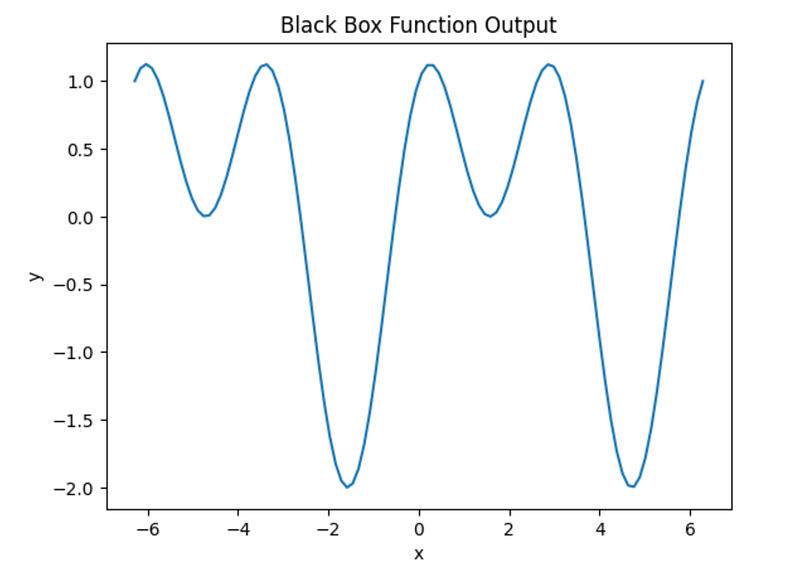
For example, let’s create a black box function that combines the sine and cosine functions to generate an output.
import numpy as np
import matplotlib.pyplot as plt
np.random.seed(42)

def black_box_function(x):
    y = np.sin(x) + np.cos(2*x)
    return y

# range of x values
x_range = np.linspace(-2*np.pi, 2*np.pi, 100)

# output for each x value
black_box_output = black_box_function(x_range)

# plot
plt.plot(x_range, black_box_output)
plt.xlabel('x')
plt.ylabel('y')
plt.title('Black Box Function Output')
plt.show()
The function values for each x value (x_range) are computed using black_box_function, and then the output is plotted.
Initial Sample
Sample outputs from function f.
# random x values for sampling
num_samples = 10
sample_x = np.random.choice(x_range, size=num_samples)

# output for each sampled x value
sample_y = black_box_function(sample_x)

# plot
plt.plot(x_range, black_box_function(x_range), label='Black Box Function')
plt.scatter(sample_x, sample_y, color='red', label='Samples')
plt.xlabel('x')
plt.ylabel('Black Box Output')
plt.title('Sampled Points')
plt.legend()
plt.show()
Modeling
Surrogate models in Bayesian optimization serve as a proxy for the true objective function. They capture the uncertainty in the function’s behavior and provide predictions or estimates of the function’s values at unobserved points within the search space. By iteratively updating the surrogate model based on observed function evaluations, Bayesian optimization guides the search towards regions of the search space likely to contain the optimal solution.
We aim to develop a model, denoted as M, that possesses the capability to not only provide predictions but also retain a measure of uncertainty associated with those predictions. For this purpose, we will adopt the following predefined interface:
- observe(M, x, y): record observations -> All
- predict(M, x): make posterior predictions -> All
- sample(M, x): sample latent function values -> Thompson
- getTail(M, v, x): the probability of exceeding x -> PI
- getImprovement(M, v, x): the integral above v -> EI
- getQuantile(M, q, x): the qth quantile -> UCB
- getEntropy(M, x): the predictive entropy -> P(ES)
The ability to execute various procedures indicates the types of approaches and acquisition functions that can be employed within the model class. The first two are applicable in all Bayesian optimization models. Additionally, for example, if you have access to the tail probabilities, you can utilize the probability of improvement (PI) method.
Gaussian Process
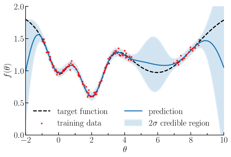
Gaussian processes (GPs) are commonly used as surrogate models in Bayesian optimization. A Gaussian process defines a distribution over functions, where any finite set of function values follows a multivariate Gaussian distribution. In the context of Bayesian optimization, a GP is used to model the unknown objective function, and it provides a posterior distribution over the function values given the observed data.

GP is fully specified by its mean function and covariance function (also called the kernel function). The mean function represents the expected value of the function at each input point, while the covariance function characterizes the relationship between different input points and controls the smoothness and behavior of the generated function.
Given a set of observed data, a GP can be used to make predictions about the function values at unobserved points. These predictions are based on the observed data and the underlying assumptions encoded in mean and covariance functions. Importantly, GPs provide a measure of uncertainty associated with these predictions, allowing for principled handling of uncertainty in predictions.
In domains with limited prior knowledge, Gaussian processes are particularly useful because they rely on the assumption that similar inputs lead to similar outputs. This makes Gaussian processes well-suited for detecting patterns and trends in the data when not much prior information is available.
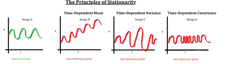
When constructing our model, we assume that it exhibits a random process, is stationary, and adheres to a Gaussian distribution. A random process refers to a mathematical model that describes the evolution of a system or phenomenon over time, where the outcomes are subject to uncertainty or randomness. Stationarity, in the context of a random process, implies that the statistical properties of the process remain constant over time. Specifically, it means that the mean, variance, and autocovariance of the process do not change with respect to time or shifts in the time origin.
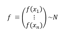
We possess an array, f, representing the values of a black box function for all its elements. We assume that this array follows a normal distribution.
The probability density function will take the form of a Gaussian density function.
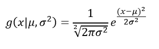
Since we assume stationarity, the joint probability distribution remains constant over time, implying it is time-invariant. The mean value of the function is m. The covariance is expected to exhibit a Gaussian shape and can be approximated using a radial basis function (RBF) kernel.
Next, we require a prediction function that aims to estimate the probability of the function f (x), given the available data we have at hand.
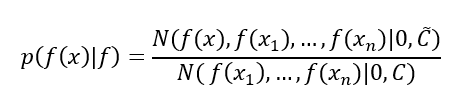
Normal distribution with 0 means and ~C covariance over normal distribution with 0 means and C covariance.
Now, we can simplify it.

k is an array of RBF kernels. C is the covariance matrix.

Using this prediction function, we can infer that, on average, the unknown function will take the value μ at x, accompanied by a variance of σ.
So, the algorithm for the surrogate function is more or less:
- Iterate through each sample value of input x for which we desire to perform an evaluation.
- Build k and f vectors using RBF kernel.
- Build matrices C and C~.
- Calculate μ and σ.
- Append μ to the predictedMu array and σ to predictedSigma arrays.
2. Calculate Omega as the mean of the black box function for sampled points.
3. Calculate Kappa = predictedMu + Omega
4. Return:
- Kappa, the mean estimate of the surrogate function
- predictedSigma, the estimate of variance from the surrogate function.
from sklearn.gaussian_process import GaussianProcessRegressor
from sklearn.gaussian_process.kernels import RBF

# Gaussian process regressor with an RBF kernel
kernel = RBF(length_scale=1.0)
gp_model = GaussianProcessRegressor(kernel=kernel)

# Fit the Gaussian process model to the sampled points
gp_model.fit(sample_x.reshape(-1, 1), sample_y)

# Generate predictions using the Gaussian process model
y_pred, y_std = gp_model.predict(x_range.reshape(-1, 1), return_std=True)

# Plot
plt.figure(figsize=(10, 6))
plt.plot(x_range, black_box_function(x_range), label='Black Box Function')
plt.scatter(sample_x, sample_y, color='red', label='Samples')
plt.plot(x_range, y_pred, color='blue', label='Gaussian Process')
plt.fill_between(x_range, y_pred - 2*y_std, y_pred + 2*y_std, color='blue', alpha=0.2)
plt.xlabel('x')
plt.ylabel('Black Box Output')
plt.title('Black Box Function with Gaussian Process Surrogate Model')
plt.legend()
plt.show()
Acquisition Function
How do we choose the next point for the surrogate function?
Acquisition functions determine the next point or set of points to evaluate in the search space. It quantifies the potential utility or desirability of sampling a particular point based on the current state of the optimization process. The purpose of the acquisition function is to balance exploration and exploitation.
It takes into account both the predicted values of the surrogate model and the uncertainty associated with those predictions. It combines these two aspects to identify points that are expected to have high objective function values and (or) high uncertainty, indicating the potential for improvement.

There are several acquisition functions used in Bayesian optimization:
- Expected Improvement (EI) selects points that have the potential to improve upon the best-observed value. It quantifies the expected improvement over the current best value and considers both the mean prediction of the surrogate model and its uncertainty.
from scipy.stats import norm

def expected_improvement(x, gp_model, best_y):
    y_pred, y_std = gp_model.predict(x.reshape(-1, 1), return_std=True)
    z = (y_pred - best_y) / y_std
    ei = (y_pred - best_y) * norm.cdf(z) + y_std * norm.pdf(z)
    return ei

# Determine the point with the highest observed function value
best_idx = np.argmax(sample_y)
best_x = sample_x[best_idx]
best_y = sample_y[best_idx]

ei = expected_improvement(x_range, gp_model, best_y)

# Plot the expected improvement
plt.figure(figsize=(10, 6))
plt.plot(x_range, ei, color='green', label='Expected Improvement')
plt.xlabel('x')
plt.ylabel('Expected Improvement')
plt.title('Expected Improvement')
plt.legend()
plt.show()
- Upper Confidence Bound (UCB) trades off exploration and exploitation by balancing the mean prediction of the surrogate model and an exploration term proportional to the uncertainty. It selects points that offer a good balance between predicted high values and exploration of uncertain regions.
def upper_confidence_bound(x, gp_model, beta):
    y_pred, y_std = gp_model.predict(x.reshape(-1, 1), return_std=True)
    ucb = y_pred + beta * y_std
    return ucb

beta = 2.0

# UCB
ucb = upper_confidence_bound(x_range, gp_model, beta)

plt.figure(figsize=(10, 6))
plt.plot(x_range, ucb, color='green', label='UCB')
plt.xlabel('x')
plt.ylabel('UCB')
plt.title('UCB')
plt.legend()
plt.show()
- Probability of Improvement (PI) estimates the probability that a point will improve upon the current best value. It considers the difference between the mean prediction and the current best value, taking into account the uncertainty in the surrogate model.
def probability_of_improvement(x, gp_model, best_y):
    y_pred, y_std = gp_model.predict(x.reshape(-1, 1), return_std=True)
    z = (y_pred - best_y) / y_std
    pi = norm.cdf(z)
    return pi

# Probability of Improvement
pi = probability_of_improvement(x_range, gp_model, best_y)


plt.figure(figsize=(10, 6))
plt.plot(x_range, pi, color='green', label='PI')
plt.xlabel('x')
plt.ylabel('PI')
plt.title('PI')
plt.legend()
plt.show()
Irrespective of the approach used, we choose the point that has the highest value on the y-axis.

num_iterations = 5

plt.figure(figsize=(10, 6))

for i in range(num_iterations):
    # Fit the Gaussian process model to the sampled points
    gp_model.fit(sample_x.reshape(-1, 1), sample_y)

    # Determine the point with the highest observed function value
    best_idx = np.argmax(sample_y)
    best_x = sample_x[best_idx]
    best_y = sample_y[best_idx]

    # Set the value of beta for the UCB acquisition function
    beta = 2.0

    # Generate the Upper Confidence Bound (UCB) using the Gaussian process model
    ucb = upper_confidence_bound(x_range, gp_model, beta)

    # Plot the black box function, surrogate function, previous points, and new points
    plt.plot(x_range, black_box_function(x_range), color='black', label='Black Box Function')
    plt.plot(x_range, ucb, color='red', linestyle='dashed', label='Surrogate Function')
    plt.scatter(sample_x, sample_y, color='blue', label='Previous Points')
    if i < num_iterations - 1:
        new_x = x_range[np.argmax(ucb)]  # Select the next point based on UCB
        new_y = black_box_function(new_x)
        sample_x = np.append(sample_x, new_x)
        sample_y = np.append(sample_y, new_y)
        plt.scatter(new_x, new_y, color='green', label='New Points')

    plt.xlabel('x')
    plt.ylabel('y')
    plt.title(f"Iteration #{i+1}")
    plt.legend()
    plt.show()
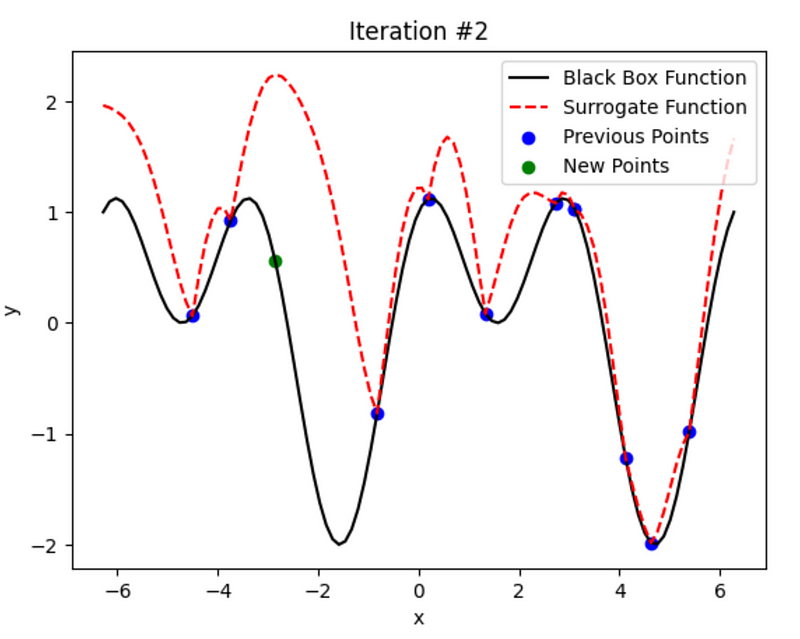
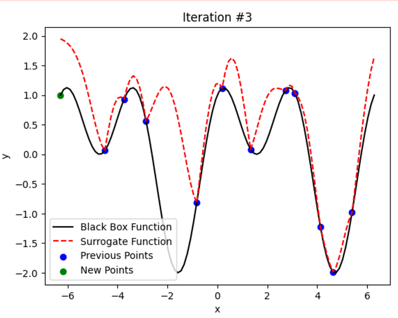

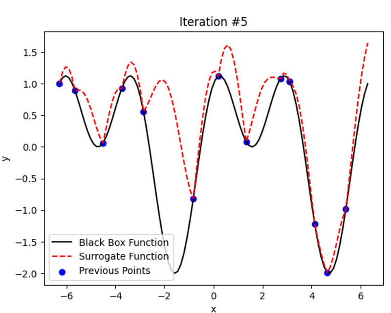
Cool, right? It keeps learning and improving in every iteration.
Bayesian optimization offers several positive aspects. One of its key advantages is the ability to optimize black-box functions that lack analytical gradients or have noisy evaluations. Employing a surrogate model, such as a Gaussian process, balances exploration and exploitation to efficiently search for the optimal solution. It provides a principled approach for iteratively selecting points that offer a good trade-off between exploring unexplored regions and exploiting promising areas.
It finds applications in various domains. It is particularly well-suited for hyperparameter tuning in machine learning. It can be used for optimizing complex simulations, experimental designs, and other scenarios where the evaluation of the objective function is costly or time-consuming.
Read More
Sources
https://nesslabs.com/exploration-exploitation-ambidextrous-mindset-success-trap


