Statistical Test on a Time Series

Time series is a collection of observations or data points measured sequentially over time. Typically, these points are recorded at regular intervals, enabling us to make reliable predictions and forecasts. Its applications range from forecasting stock prices and predicting weather patterns to analyzing medical data and optimizing supply chain management. By delving into historical patterns and trends, we gain valuable insights that can enhance productivity and decision-making in diverse fields.

Time series forecasting involves utilizing a model to anticipate future values based on patterns and trends observed in historical time series data. Time series analysis plays a crucial role in machine learning. By analyzing time-series data, machine learning algorithms can identify seasonal patterns, trends, and other underlying structures, which are then leveraged for forecasting future observations. Intervals of the Time Series Data

Yearly- GDP, Macro-economic series

Quarterly- Revenue of a company.

Monthly- Sales, Expenditure, Salary

Weekly- Movie theater ticket sales, Price of Petrol and Diesel

Daily- Closing price of stock, Sensex value, daily transaction of ATM machine

Hourly- AAQI, Weather data

Forecasting, as you rightly pointed out, relies on models trained on historical data to make predictions about future data points. These models capture the relationships and patterns present in the time series, allowing us to anticipate potential outcomes with a certain level of confidence. This predictive capability enables businesses and organizations to plan, make informed decisions, and allocate resources effectively based on anticipated future trends and patterns.

It’s essential to recognize that forecasting doesn’t provide an exact prediction of the future. Instead, it offers an estimated projection based on past data, offering insights into potential future outcomes. This estimation helps us make informed decisions and prepare for various scenarios based on the historical behavior of the time series data.

Time Series Types

a) Univariate Time Series: A univariate Time series is a series of data with a single time dependent variable like Demand for a product at a certain time interval.

b) Multivariate Time Series: A multivariate time series data contains more than one-time dependent variable. Each variable depends on the past values and on other variables. This dependency is used for forecasting future values.

Commonly Used Terms:

• Level: This represents the base value of the series if it followed a straight line, indicating its average or baseline behavior.
• Trend: The trend component captures the overall linear increasing or decreasing behavior of the series over time. It reflects the long-term direction in which the series is heading.
• Seasonality: Seasonality refers to the repeating patterns or cycles of behavior exhibited by the series over time. These patterns often occur at regular intervals, such as daily, weekly, monthly, or yearly cycles.
• Noise: Noise, also known as residual or error, represents the variability in the observations that cannot be explained by the model. It includes random fluctuations and irregularities in the data not accounted for by trends or seasonal components.
• Cyclicity: Cyclicity in time series refers to the presence of recurring patterns or fluctuations that occur over longer time frames than typical seasonal variations. Unlike seasonal patterns, which occur at fixed intervals (e.g., daily, weekly, monthly), cyclical patterns do not have a predetermined frequency or duration.
• Seasonal period: Seasonal period is the frequency number in the data that repeat over a specific duration, such as days, weeks, months, or years; for Annual it is 1, Quarterly 4, Monthly 12 and weekly 52 for daily observations data
• Stationary: Stationarity is a key concept in time series analysis, and it refers to a series whose statistical properties remain constant over time. Specifically, in a stationary time series: 1) The mean of the series remains constant and does not exhibit any trend or systematic change over time. 2) The variance of the series remains constant, indicating that the spread or dispersion of data points around the mean does not change over time. 3) The covariance between two observations at different time points remains constant, indicating that the relationship between observations does not change over time. 4) The standard deviation, being derived from the mean and variance, also remains constant.

In simpler terms, a stationary time series does not exhibit any trend or seasonal patterns, and its statistical properties remain stable over time. This makes it easier to model and analyze the series, as the relationships between data points are consistent and predictable. Types of stationary:

• Strict Stationary — Follows mathematical definition of a stationary process. Mean, variance & covariance are not a function of time.
• Seasonal Stationary — Series exhibiting seasonality.
• Trend Stationary — Series exhibiting trend.

Type of Seasonality:

• Additive Seasonality: Additive seasonality occurs when the seasonal fluctuations in the data have a consistent magnitude over time. In other words, the seasonal component is added to the overall trend of the series.
• Multiplicative Seasonality: Multiplicative seasonality occurs when the seasonal fluctuations in the data increase or decrease in proportion to the series’ overall trend. This means that the seasonal component is multiplied by the overall trend.
• Weekly Seasonality: Some time series exhibit weekly seasonality, where patterns repeat weekly. For example, sales data might show higher volumes on weekends compared to weekdays.
• Monthly Seasonality: Monthly seasonality refers to patterns that repeat monthly. For instance, retail sales might experience peaks around the end of each month due to paydays.
• Quarterly Seasonality: Quarterly seasonality involves patterns that repeat every quarter of the year. This is often observed in financial data or economic indicators.
• Yearly Seasonality: Yearly seasonality refers to patterns that repeat annually. For example, retail sales might experience spikes during holiday seasons such as Christmas or back-to-school periods.
• Non-Integer Seasonality: In some cases, seasonal patterns may not follow exact integer multiples of weeks, months, quarters, or years. This can occur due to various factors such as irregular holidays or shifts in consumer behavior.
• Multiple Seasonality: Some time series may exhibit multiple seasonal patterns simultaneously. For example, a retail store might experience weekly and yearly seasonality and additional seasonal patterns related to specific events or promotions.

Type of Trend:

• Linear Trend: A linear trend occurs when the data points exhibit a constant increase or decrease over time at a relatively constant rate. It can be represented by a straight line when plotted on a graph.
• Exponential Trend: An exponential trend occurs when the data points exhibit an increasing or decreasing rate of change over time. Unlike a linear trend, the rate of change is not constant but instead accelerates or decelerates exponentially.
• Logarithmic Trend: A logarithmic trend occurs when the rate of change in the data decreases over time, resulting in a curve that flattens out gradually. This type of trend is often observed when the data approaches a limiting value or saturation point.
• Seasonal Trend: A seasonal trend involves regular, recurring patterns or cycles in the data that occur over fixed intervals of time, such as days, weeks, months, or years. These patterns may be influenced by factors such as seasons, holidays, or other periodic events.
• Cyclical Trend: A cyclical trend represents longer-term fluctuations in the data that are not necessarily of fixed duration or frequency. Unlike seasonal trends, cyclical trends do not have a fixed pattern or period and may result from economic, business, or other systemic factors.
• Random or Irregular Trend: Sometimes, time series data may exhibit random or irregular fluctuations that do not follow any discernible trend or pattern. These fluctuations may result from random noise, measurement errors, or other unpredictable factors.

Statistical Test:

Visual inspection is often the first step in assessing stationarity in time series data. Trends and seasonal components can often be visually identified through plots such as time series plots, scatter plots, and seasonal subseries plots.

In addition to visual inspection, statistical tests provide more objective methods for detecting stationarity.

• Augmented Dickey-Fuller (ADF) Test: The ADF test is a hypothesis test used to determine whether a unit root is present in a time series dataset. A unit root indicates non-stationarity, implying that the series possesses a stochastic trend.

Null Hypothesis: Series is non-stationary or series has a unit root

Alternate Hypothesis: Series is stationary or series has no unit root

The critical values are determined based on the chosen significance level (usually 0.05), and if the test statistic is less than the critical value and the p-value is less than 0.05, the null hypothesis is rejected, indicating that the series is stationary. Rejecting the null hypothesis suggests that the series does not exhibit a unit root and is therefore stationary, meaning it lacks a time-dependent structure and has stable statistical properties over time. This is an essential step in time series analysis, as stationary data are easier to model and forecast accurately compared to non-stationary data.

from statsmodels.tsa.stattools import adfuller
def ADF_test (series):    
    adf = adfuller(series)
    print('ADF Test Result')
    print("Test statistic: {}".format (adf[0])) 
    print("p-value: {}".format (adf[1]))
    print ("Critical values : ")
    for key, value in adf[4].items():
        print("{} : {}".format(key, value))
    if (adf[1] <= 0.05):
        print('Reject the null hypothesis')
        print('Series is Stationary')
    else:
        print('Failed to reject the null hypothesis')
        print('Series is Non-Stationary')

• Kwiatkowski-Phillips-Schmidt-Shin (KPSS) Test: However, KPSS is used to test for a trend in a time series dataset. Unlike the ADF test, which assumes a stochastic trend, the KPSS test assumes a deterministic trend.

Null Hypothesis: The process is trend stationary.

Alternate Hypothesis: The series has a unit root (series is not stationary).

If the null hypothesis is failed to be rejected, this test may provide evidence that the series is trend stationary. If the Test Statistic < Critical Value and p-value is less than 0.05 — Fail to Reject Null which means, time series does not have a unit root, meaning it is trend stationary.

from statsmodels.tsa.stattools import kpss
def KPSS_test (series):
    print ("KPSS Test Result")
    kpss_test = kpss(series, regression='ct')
    print("Test statistic: {}".format (kpss_test[0])) 
    print("p-value: {}".format (kpss_test[1]))
    print ("Critical values :")
    for key, value in kpss_test[3].items():
        print("{} : {}".format(key, value))                             
    if(kpss_test[1] < 0.05):
        print('Series is Non-Stationary')
    else:
        print('Series is Stationary')

Note: It is always better to check both the tests, so that it can be ensured that the series is truly stationary. Possible outcomes of applying these stationary tests are as follows:

Case 1: Both tests conclude that the series is not stationary — The series is not stationary

Case 2: Both tests conclude that the series is stationary — The series is stationary

Case 3: KPSS indicates stationarity and ADF indicates non-stationarity — The series is trend stationary. Trend needs to be removed to make series strict stationary. The detrended series is checked for stationarity.

Case 4: KPSS indicates non-stationarity and ADF indicates stationarity — The series is difference stationary. Differencing is to be used to make series stationary. The differenced series is checked for stationarity.

• Kruskal-Wallis Test: The idea of using the Kruskal-Wallis test for time series analysis is interesting! Main reason to say that,

1.Non-parametric approach: This test is a non-parametric test which means it doesn’t require any specific distribution for your data. This is crucial for time series data, which often exhibits seasonality and may not be normally distributed.

2.Median focused: The test compares the medians of different groups, making it sensitive to shifts in the center of the distribution across seasons. This can be particularly useful if your seasonal variations are not symmetrical.

3.Identifies differences between groups: In the context of time series, the groups can represent different seasons (e.g., winter, spring, summer, fall). The KW test can tell you if there’s a statistically significant difference in the medians of these seasonal groups.

For this test be careful about your seasons, are they equal length (e.g., quarters) or based on natural cycles (e.g., rainfall patterns). The Kruskal-Wallis test provides evidence of seasonality if the p-value associated with the test statistic is below a chosen significance level (e.g., 0.05). A low p-value suggests that there are significant differences between the groups, supporting the existence of seasonality. The Kruskal-Wallis Test has the null and alternative hypotheses as discussed below:

Null Hypothesis: median is the same for all the data groups.

Alternative Hypothesis: median is not equal for all the data groups.

from scipy.stats import kruskal
def seasonality_test(series):
    seasonal = 0
    idx = np.arange(len(series.index)) % 12
    H_statistic, p_value = kruskal(series, idx)
    if p_value <= 0.05:
        seasonal = 1
        return {"RESPONSE": "success",
                "data": (seasonal, "The series has seasonality")
                }
    return {"RESPONSE": "success",
            "data": (seasonal, "No seasonality found in the series")
            }

• Hodrick-Prescott Filter: The Hodrick-Prescott (HP) filter refers to a data-smoothing technique. The HP filter acts as a data smoothing technique, removing high-frequency fluctuations (short-term ups and downs) associated with business cycles. In practical applications, this filter is used to achieve two main goals: smoothing the data by removing short-term noise and detrending the data by extracting the long-term trend component. So basically Hodrick-Prescott filter is indeed a tool used in time series analysis to separate the data into two main components: trend and cycle.

from statsmodels.tsa.filters.hp_filter import hpfilter
def hodrick_prescott(series, lamb):
    df = series.to_frame()
    cycle, trend = hpfilter(series, lamb= lamb)
    df['cycle'], df['trend'] = cycle, trend
    return df

• Mann-Kendall Test: The Mann-Kendall (MK) test is a powerful tool for detecting trends in time series data, and it offers some distinct advantages:

1.Non-parametric approach: Like the Kruskal-Wallis test, the MK test is non-parametric. It doesn’t require the data to follow a specific distribution.

2.Monotonic Trends: This test focuses on monotonic trends, which means the data consistently increases or decreases over a certain period. Also, it is helpful for identifying both upward and downward trends, regardless of linearity.

3.Seasonal /Non-seasonal: Although the main concept of MK test is designed for non-seasonal trends, there are ways like the Seasonal Mann-Kendall test that can specifically detect seasonal trends. These variations account for the cyclical nature of the data and identify trends within each season.

import pymannkendall as mk
def MK_Test(series, seasonal):
    if seasonal == False:
        data_mk = mk.original_test(series)
        trend = data_mk[0]
        p_value = data_mk[2]
    else:
        data_mk_seasonal_test = mk.seasonal_test(series, period= 12)
        trend = data_mk_seasonal_test[0]
        p_value = data_mk_seasonal_test[2]
    
    if trend == "decreasing" or trend == "increasing":
        trend = "Present"
        return p_value, trend
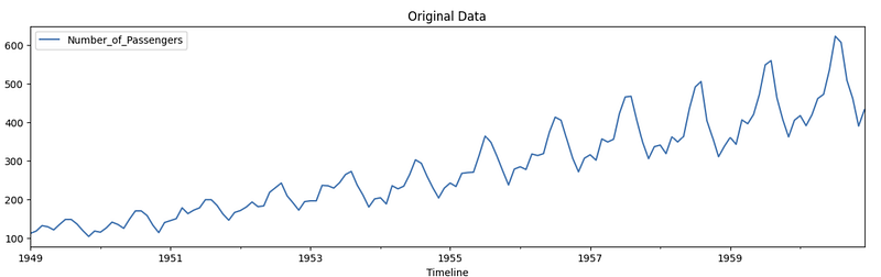
    return p_value, trend

Statistical Test Result:

For test used Airline passengers from 1949 to 1960 monthly data. This dataset can be used to perform univariate time series analysis. link

Also check this link to find the test results.