Summary

The content describes the negative binomial distribution through the story of Dave, a basketball player tracking the number of attempts needed to make five three-point shots, and explains its assumptions, formula, and real-world applications.

Abstract

Dave, an avid basketball player, uses the negative binomial distribution to analyze his shooting performance by tracking the number of attempts to make five shots. This distribution is shown to be a valuable tool for predicting the number of trials needed to achieve a fixed number of successes, given the probability of success remains constant and each trial is independent. The negative binomial distribution provides insights into Dave's average performance and the variation in his results, enabling him to set realistic expectations and monitor improvements. The content further details the key assumptions, mathematical formula, and various practical examples where this distribution can be applied, such as in production quality control, customer service, insurance claim analysis, disease outbreak monitoring, and e-commerce conversion tracking.

Opinions

Dave finds the negative binomial distribution useful for understanding his basketball shooting performance and setting realistic goals.
The author suggests that the negative binomial distribution can be applied to a variety of real-world scenarios beyond sports, indicating its broad utility.
The story implies that visualizing the distribution through charts can provide clearer insights into performance patterns and probabilities.
The content conveys that the negative binomial distribution is particularly relevant for processes involving a fixed number of successes and variable numbers of trials or failures.

Statistical Stories - Negative Binomial Distribution

Below is a story and some additional information to help you understand the negative binomial distribution. Visit statisticalstories.xyz/negative-binomial to read all this and play with some interactive visualizations to help you fully understand this distribution.

The Probability Mass Function for the Negative Binomial distribution

The Story

Once upon a time, there was a man named Dave who loved playing basketball. He had a goal of making as many three-point shots as possible in a game. One day, he decided to keep track of his shots and count how many attempts it took for him to make five shots.

As Dave started playing, he quickly realized that he didn’t always make a shot on his first try. Sometimes it took him two attempts, sometimes three, and occasionally even more. Curious about this pattern, Dave decided to analyze his shooting performance using something called the negative binomial distribution.

Dave understood that the negative binomial distribution could help him predict how many attempts it would take for him to make a certain number of shots. In this case, his target was five made shots. The negative binomial distribution focuses on the number of trials or attempts needed until a specific number of successes occur.

So, Dave began collecting data during his basketball practices. He recorded the number of attempts it took him to make five shots each time. After several rounds, he had a list of results.

As he analyzed the data, Dave noticed that the probability of making a shot on each attempt remained constant. It was like flipping a coin with a fixed probability of heads or tails. Sometimes he made a shot, and sometimes he didn’t.

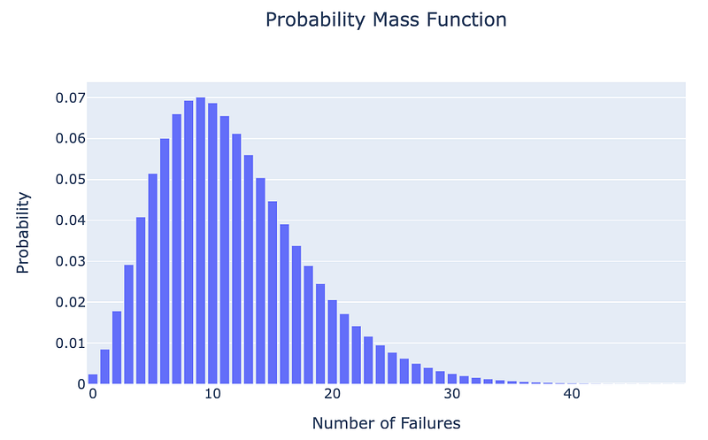
To understand the negative binomial distribution better, Dave decided to visualize it. He created a chart where the x-axis represented the number of attempts required to make five shots, and the y-axis represented the probability of this requirement. The shape of the chart resembled a skewed curve.

When Dave examined the chart, he noticed a few interesting things. Firstly, the peak of the curve indicated the average number of attempts it took for him to make five shots. Secondly, the curve gradually declined as the number of attempts increased, showing that the probability of requiring many attempts was less likely.

Dave realized that the negative binomial distribution helped him understand the likelihood of achieving his goal based on his shooting performance. It gave him insights into the average number of attempts it took for him to make five shots, as well as the variation in his performance from game to game.

Armed with this knowledge, Dave could set realistic expectations for himself. He understood that if his shooting skills improved, he could expect to make five shots in fewer attempts. Conversely, if he was having an off day, he might need more attempts to reach his target.

As Dave continued playing basketball and tracking his shooting performance, he found the negative binomial distribution to be a useful tool in understanding his progress. It allowed him to set goals, monitor his improvement, and adjust his strategy accordingly.

Assumptions

1. Independent and Identically Distributed (IID) Trials: Each trial or attempt is independent of the others.

2. Fixed Probability of Success: The probability of success (e.g., making a shot) remains constant in each trial.

3. Discrete Outcomes: The outcome is a discrete (i.e. integer) variable, instead of a continuous variables.

Formula

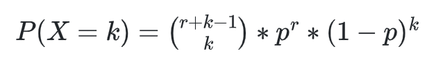
Where:

P(X = k): The probability that the random variable X takes on the value k.
r: The number of successes needed before the experiment is complete.
k: The number of failures until the required number of successes is reached.
p: The probability of success in each trial.
(1 − p): The probability of failure in each trial.
(r + k − 1) over k: The binomial coefficient, also known as “n choose k.” It calculates the number of ways to choose k failures out of (r + k −1) trials.

Examples

1. To model the number of defects or faulty units in a production process before a specified number of acceptable units is produced.

2. To analyze the number of customer complaints or service requests received before a certain number of satisfactory resolutions is achieved.

3. To estimate the number of claims an insurance company receives before a predetermined number of high-cost claims occur.

4. To model the number of disease outbreaks or infections until a certain number of hospitalizations is reached.

5. To model the number of website visits before a certain number of purchases occur.