A Baby Robot’s Guide To Reinforcement Learning

State Values and Policy Evaluation in 5 minutes

An Introduction to Reinforcement Learning

This is a summary of the article State Values and Policy Evaluation. It distils all of the key terms and theory from that article down into a single cheat-sheet that can be read in 5 minutes or less. With that in mind, we’d better get started…

You can also open this article as a Jupyter Notebook on Binder which allows you to run the associated code samples using the Baby Robot Custom Gym Environment.

Reinforcement Learning

Reinforcement Learning can be considered to be a problem that takes place in an environment that consists of multiple, independent, states.

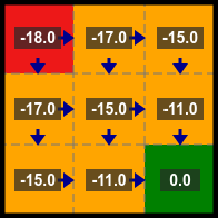
A simple example of this would be a grid world, where each square in the grid represents a state:

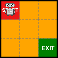
State

A unique, self-contained, stage in the environment that defines the current situation. Each state is independent of previous states, which means you don’t need to know or remember what has happened before.

Episode

One complete execution of the environment.

Terminal State

The final state in an environment where the episode ends.

Agent

The agent is the thing that interacts with the environment and that makes decisions on how to move through the environment. In our case Baby Robot is the agent.

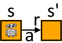
To move from one state s to the next state s’ (read as s-prime) the agent takes an action a. As a result of taking this action it receives a reward r.

Reward

The numerical value used to measure performance. It can be expressed as a penalty by making it negative. The more negative the worse the performance.

Expected reward for a state-action pair

The expected reward can be thought of as the average reward and is used if the reward given for a particular action can vary.

At time ‘t -1’, starting in a particular state s and taking action a, the expected reward that’s received at the next time step is a function of the current state and action.

Return ‘Gₜ’

The total amount of reward accumulated over an episode, starting at time t is equal to the sum of future rewards:

Policy

The strategy that is used by the agent to choose an action in a state. In equations the policy is typically represented by ‘π’.

Greedy Policy

Selects the action with the highest immediate reward.

Reinforcement Learning can be split into two distinct parts, the Prediction Problem and the Control Problem:

Prediction Problem

Evaluate the performance of an agent.

State Value

A measure of how good it is to be in that state. Given by the expected reward that can be obtained from starting in that state and then following the current policy for all future states.

The value for state s under policy π is the expected return:

For a deterministic policy, where a single action is always selected in each state and when you’re guaranteed of getting the same reward and ending up in the same next state, the value of a state is simply the immediate reward plus the value of the next state:

For a stochastic policy, where multiple actions are possible, π(a|s) represents the probability of taking action a from state s under policy π.

In this case the state value is given by the sum of each action’s reward multiplied by the probability of taking that action:

Dynamic Programming

Splits the problem into simpler sub-problems. In this case the state value is calculated by splitting the problem into 2 parts: the immediate reward and the value of the next state.

State values are calculated using the values of other states. As a result you only need to look one step ahead and don’t need to know all of the rewards accumulated during the episode.

Iterative Policy Evaluation

By repeatedly applying the above equation for the state value the converged state value can be calculated.

The algorithm for this is:

• Start with all state values set to zero.
• Do a sweep of all states to calculate the state values (using the above equation).
• Repeat until convergence.

Control Problem

Modify the policy to improve performance.

Policy Improvement

After the state values have been calculated act greedily with respect to these values to form a new policy (i.e. choose the action which will take you to the next state that has the greatest state value).

Discounted Rewards

Progressively reduce the contribution of rewards from future time steps by using a discount factor γ (gamma), where 0 ≤ γ ≤ 1.

This allows the calculation of state values for deterministic policies that may not terminate. A value of 0.9 is commonly used as the discount factor.

The value of state s under policy π with discounted future rewards is given by:

Summary

We’ve now covered all of the basics of Reinforcement Learning (RL) and all in record time!

We concluded our introduction with an equation that’s a cut-down version of the Bellman Equation, the key equation in Reinforcement Learning. In Part 2 of this series we’ll look at the full Bellman Equation and examine Markov Decision Processes which are another core concept of RL.

For a more detailed explanation of all of the topics covered in this article check out the original post: