Summary

The provided content discusses the application of the Extended Kalman Filter (EKF) for state estimation in robotics, particularly for self-driving vehicles.

Abstract

The Extended Kalman Filter (EKF) is a crucial algorithm for state estimation in non-linear systems, such as robotic cars. It enhances the accuracy of state estimation by combining noisy sensor measurements with predicted measurements. The EKF is part of a broader category of filters known as Kalman filters, adapted for non-linear systems. In the context of a robotic car, the EKF estimates the car's position and orientation by considering its linear and angular velocities within a global coordinate frame. The process involves a state-space model to predict the car's next state and an observation model to infer sensor measurements. These models use mathematical representations, including trigonometric functions and Jacobian matrices, to account for non-linearities. The EKF operates in two phases: prediction, which estimates the state and covariance matrix, and update, which incorporates actual sensor measurements to refine the state estimate. Despite its effectiveness, the EKF is subject to linearization errors, which can be problematic in high-speed scenarios, leading to potential overconfidence in erroneous estimates.

Opinions

The author suggests that EKF is essential for accurate state estimation in robotics due to its ability to handle non-linear motion systems.
Sensor fusion, facilitated by the EKF, is highlighted as a critical process for improving state estimates by smoothing out noisy sensor data.
The author emphasizes the importance of the Jacobian matrix in linearizing non-linear equations within the EKF framework.
The EKF is portrayed as a practical solution for real-time state estimation in self-driving cars, despite its inherent limitations.
The author indicates a preference for the Unscented Kalman Filter (UKF) as a superior alternative to the EKF, due to its ability to better handle non-linearities and reduce linearization errors.
The author promotes an AI service, ZAI.chat, as a cost-effective alternative to ChatGPT Plus (GPT-4), suggesting its utility and value for those interested in AI applications.

State Estimation using Extend Kalman Filter (EKF) for robotics

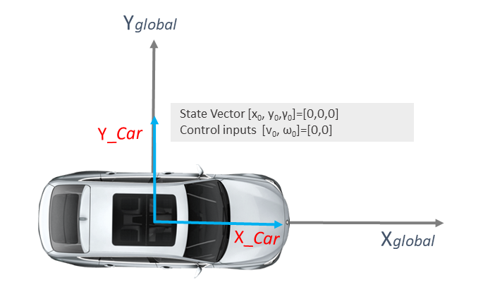
EKF was designed to enable the Kalman filter to apply in non-linear motion systems such as robots. EKF generates more accurate estimates of the state than using just actual measurements alone. In this post, we will briefly walk through the Extended Kalman Filter, and we will get a feel of how sensor fusion works. In order to discuss EKF, we will consider a robotic car (self-driving vehicle in this case). We can model this car as illustrated in the figure below in a global coordinate frame with coordinates: Xglobal, Yglobal, and Zglobal (face upwards). The X_car and Y_car coordinates belong to the coordinate frame of the car which is moving with a linear velocity (V) and angular velocity (ω). The yaw angle (γ) measures how much the car is rotated around the global z-axis.

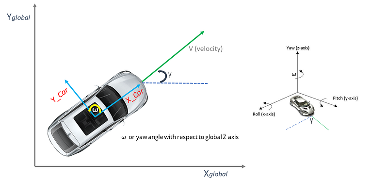
EKF is seen in almost every field of robotics for estimating states. The goal of EKF is to smooth out the noisy sensor measurements of the car for better state estimation. State here means where is the car located? and how much it is rotated? In order to estimate the state of the vehicle, EKF combines the noisy sensor measurements with the predicted sensor measurement to generate an optimal estimation. However, to understand how EKF functions we need to know about two mathematical building blocks of EKF:

State-Space Model
Observation Model

1. State Space or motion model

Using the state-space model we can predict the next state of the car. It is also known as the state transition model that represents the motion of the car or a robot from the current to the next time-step. For example, it shows how the current state of our car changes based on the control given to the car [Linear velocity (V) and angular velocity (ω)] using Steering, throttle and brakes. The steering impacts the ω, whereas throttle and brakes impact the linear velocity (V). From now on, we will represent the state of the car at time t as [xt, yt, γt] and the control inputs as [vt, ωt]. We are using these terms in order to avoid confusion while going through the literature on the internet. Now let's derive the velocity components of the car in terms of the global reference frame.

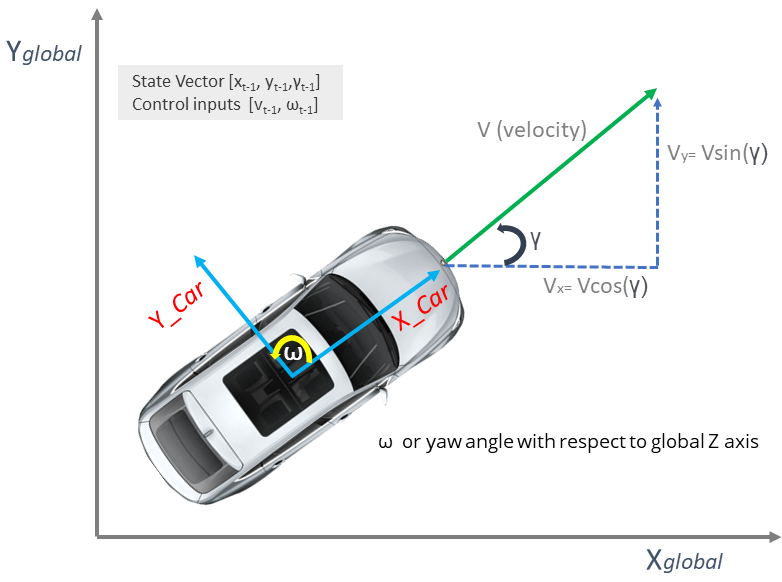
As shown in the figure above, by applying trigonometry we have Vx=Vcos(y) and Vy=Vsin(y) with angular velocity ω. Now, given our initial state [xt-1, yt-1,γt-1], we can estimate the next state [xt, yt,γt] as follows:

Note: we start from t=1 so that the initial state is [x0, y0, γ0]

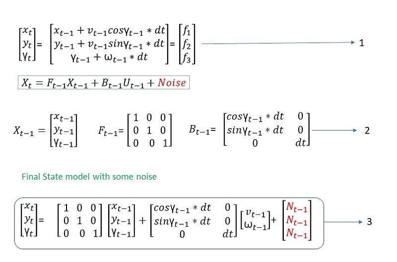
In the above figure, we have mathematically described the motion of the robot car. In equation 1, at time dt the car would have moved up to some distance. Since we know that distance can be written as the product of velocity (v) and time (t), equation 1 can be obtained easily. Each of the terms (f1, f2 and f3) will be used to compute the jacobian matrix F. Here we use Jacobian since we need to linearize the non-linear equations which have cosine and sine terms.

In equation 2, Xt represents the motion model at time t. The F and B are the jacobian matrices, and in our case, F is an identity matrix since the car moves only based on input controls i.e. Linear and angular velocity. But, it is not always an identity matrix. Think about the situation of an aeroplane. In an aeroplane, gravitation force acts, and if we don’t provide the control inputs then it will fall and crash. So, in such a case F is not Identity.

Finally, equation 3 represents the complete state-space model with noise terms added

2. Observation model

We have an estimate of the car using the state-space or the motion model. Now we will smooth out the sensor measurements to generate a better estimate of the current state of the robot car (This is called SENSOR FUSION). At first, our state model predicts the next state, and then the Observation model takes the predicted input [xt, yt, Yt] of the state model to generate (infer) new measurements.

Why this is necessary?

Imagine a situation when you are on a self-driving car and the sensors are breaking down. Now we want the car to move to the goal location. In such a situation, the observation model can predict what would be sensor measurement at some time in the future. So, even if the car sensors break downs and produce erroneous data, the observation model tries to reduce the error.

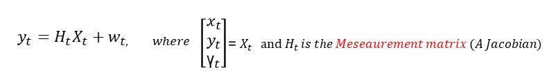
yt is n-dimensional which represents n number of sensor measurement. The w is the noise with respect to each of the sensors. H is the measurement matrix which converts predicted state estimate to a predicted sensor measurements

We have made the following two assumptions based on the above discussions.

State Model estimates the state of the robot based on the control inputs
Observation model infers sensor measurement using the predicted state

Extended Kalman Filter-(EKF)

Now think about the self-driving car that has sensors mounted on it and provides sensor measurement. The EKF computes the weighted average of these actual sensor measurements at the current time step t and predicted sensor measurements (as we discussed above) to generate a better current state estimate. The EKF has two phases: Prediction and update (shown in the figure below)

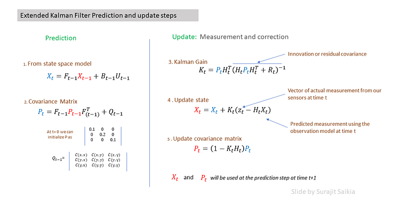
EKF prediction and update steps (created by Surajit Saikia)

The above figure shows the prediction and update steps of the Extended Kalman Filter. At the prediction step, we first estimate the state (Xt) using the state-space or the motion model (I have removed the noise terms just to make it look clean). After that, we obtain the state covariance matrix P at time t using the previous covariance matrix P at time t-1. The state covariance matrix holds the uncertainty of the states. However, for the first iteration, we don't have the covariance matrix, so we initialise it as shown in the figure above. In addition, the initial state vector of the car would be zero along with the control commands.

Matrix F is the transition matrix, which is used to predict the next value x and the covariance matrix P. Matrix Q is the process noise covariance matrix. The dimension of Q is (number of states * number of states), and in our case, it is 3x3. This Q term is important since the state measurement has noises and we need to measure the variance.

Rt (sensor measurement noise covariance matrix)

K indicates how much the state and covariance of the state predictions should be corrected due to the new actual sensor measurements (zt). If the sensor noise is high (residual covariance is high), the value of K tends to zero and sensor measurements will be ignored. If the predicted noise is high, then K approaches 1, and we will rely on the sensor measurement. Finally, Xt and Pt are updated and are used in the next step of prediction. In other words, Kalman gain (K) contains information on how much weight to place on the current prediction X and current observed measurement z that will result in the final fused updated state vector x and process covariance matrix P.

So, we are done with the EKF. However, EKF has a linearization error which basically depends on how non-linear the function is and the distance of the operating point that is being used for linearization. The linearization error can have a catastrophic effect on self-driving cars since it causes the estimator to be overconfident in the wrong answer. In addition, deriving the Jacobian is a tedious and error-prone process. If the self-driving car moves very fast, then more is the linearization error. Next, we will go through the Unscented KALMAN filter that addresses the above limitations.

LinkedIn: https://www.linkedin.com/in/surajit-saikia-55b717101/