Stat Stories: Normalizing Flows as an Application of Variable Transformation

Generative Models for Tractable Distributions

In my previous episodes of the Stat Stories series, I talked about methods of variable transformation to generate new distribution. The discussion on the variable transformation, both for univariate and multivariate distributions leads to Normalizing Flows.

I recommend reading the discussion on variable transformation for generating new distributions as a prerequisite to understanding Normalizing Flows.

Introduction

A big challenge in statistical machine learning is to model a probability distribution if we are already given samples from some distribution. Normalizing flows was first coined by Tabak and VandenEijnden [2010] and Tabak and Turner [2013] in the context of clustering, classification, and density estimation.

Definition: Normalizing Flows can be defined as a transformation of a simpler probability distribution such as uniform distribution into a complicated distribution such as one that can give you a random sample of cat images by applying a sequence of invertible transformations.

As a result of a sequence of invertible transformations, we can obtain new families of distributions by selecting an initial density function that is simple and then chaining together a number of parametrized, invertible and differentiable transformations. This way, we can obtain samples corresponding to new densities.

One thing to note is that in the context of Normalizing flows, transformation is parametrized as compared to my initial discussion in https://rahulbhadani.medium.com/stat-stories-variable-transformation-to-generate-new-distributions-d4607cb32c30 where the transformation I used doesn’t contain any parameter. However, the idea stays the same.

Let’s look at the formula of the variable transformation once again:

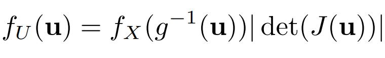
where U is a multivariate random vector for the new distribution and X is the multivariate random vector for the original initial distribution. J is the Jacobian. In the context of Normalizing flows, the new density function fᵤ is called pushforward, and g is called the generator. This movement from the initial simple density to the final complicated density is called the generative direction. The inverse function g⁻¹ moves in the opposite direction called the normalizing direction. That is why the overall process of transformation is called Normalizing flows. To generate a data point corresponding to U, apply the transformation u = g(x).

For a more detailed and formal approach to the definition of Normalizing Flows, I recommend looking at Normalizing Flows: An Introduction and Review of Current Methods (https://arxiv.org/pdf/1908.09257.pdf).

Applications of Normalizing Flows

While other statistical methods such as Generative Adversarial Networks (GAN) and Variational AutoEncoders (VAN) have been able to perform dramatic results on difficult tasks such as learning distributions of images, and other complicated datasets, they do not allow evaluation of density estimation and calculation of probability density of new data points. In such a sense, Normalizing Flows proves to be eloquent. The method can perform density estimation and sampling as well as variational inferences.

Density Estimation and Sampling

Consider a transformation u = g(x ; θ), i.e. , g is parametrized by parameter vector θ. Initial probability density function fₓ is parametrized by a vector φ, i.e. fₓ(x | φ). If we have sample points 𝓓 corresponding to the desired distribution F_U, then we can perform log-likelihood estimation of parameters Θ = (θ, φ) as follows:

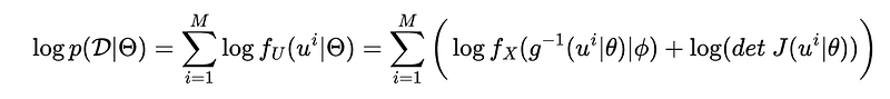
During the neural network training, parameters evolve to maximize the log likelihood. There are a number of choices that can be made in choosing a loss function such as adversarial loss, but the choice entirely depends on the application.

I will discuss variational inference separately from a broader context in an upcoming article. Be sure to subscribe to my email list to receive a notification about that. In the meantime, let’s look at some code using Python.

Example

For the example, I will use the Flowtorch library that can be installed using

pip install flowtorch

While in my previous articles, I derived the transformed density function by hand, we can use Flowtorch’s implementation of Normalizing Flows for learnable transforms and estimate density estimation.

Let’s look at the samples of two concentric circle dataset

import numpy as np
from sklearn import datasets
from sklearn.preprocessing import StandardScaler

n_samples = 1000
X, y = datasets.make_circles(n_samples=n_samples, factor=0.5, noise=0.05)
X = StandardScaler().fit_transform(X)

plt.title(r'Samples from $p(x_1,x_2)$')
plt.xlabel(r'$x_1$')
plt.ylabel(r'$x_2$')
plt.scatter(X[:,0], X[:,1], alpha=0.5)
plt.show()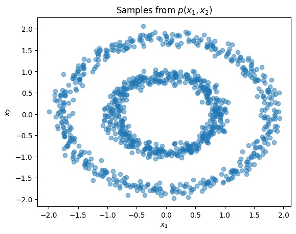

plt.subplot(1, 2, 1)
sns.distplot(X[:,0], hist=False, kde=True,
bins=None,hist_kws={'edgecolor':'black'}, kde_kws={'linewidth': 2})

plt.title(r'$p(x_1)$')
plt.subplot(1, 2, 2)
sns.distplot(X[:,1], hist=False, kde=True, bins=None, hist_kws={'edgecolor':'black'}, kde_kws={'linewidth': 2})

plt.title(r'$p(x_2)$')
plt.show()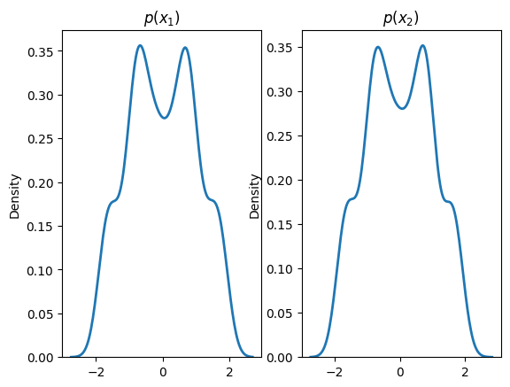

We can learn the marginal transform bij.Spline. Knots and derivatives of splines act as parameters that can be learned using stochastic gradient descent:

dist_x = torch.distributions.Independent(
  torch.distributions.Normal(torch.zeros(2), torch.ones(2)), 
  1
)
bijector = bij.Spline()
dist_y = dist.Flow(dist_x, bijector)

optimizer = torch.optim.Adam(dist_y.parameters(), lr=1e-2)
steps = 5000

X = torch.Tensor(X)
for step in range(steps):
    optimizer.zero_grad()
    loss = -dist_y.log_prob(X).mean()
    loss.backward()
    optimizer.step()

    if step % 200 == 0:
        print('step: {}, loss: {}'.format(step, loss.item()))

Now, we can plot samples from the transformed distribution after learning:

X_flow = dist_y.sample(torch.Size([1000,])).detach().numpy()
plt.title(r'Joint Distribution')
plt.xlabel(r'$x_1$')
plt.ylabel(r'$x_2$')
plt.scatter(X[:,0], X[:,1], label='data', alpha=0.5)
plt.scatter(X_flow[:,0], X_flow[:,1], color='firebrick', label='flow', alpha=0.5)
plt.legend()
plt.show()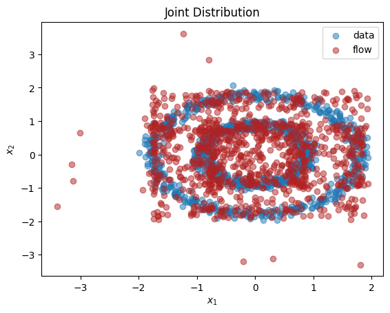

and we can plot the learned marginal distribution:

plt.subplot(1, 2, 1)
sns.distplot(X[:,0], hist=False, kde=True,
             bins=None,
             hist_kws={'edgecolor':'black'},
             kde_kws={'linewidth': 2},
             label='data')
sns.distplot(X_flow[:,0], hist=False, kde=True,
             bins=None, color='firebrick',
             hist_kws={'edgecolor':'black'},
             kde_kws={'linewidth': 2},
             label='flow')
plt.title(r'$p(x_1)$')
plt.subplot(1, 2, 2)
sns.distplot(X[:,1], hist=False, kde=True,
             bins=None,
             hist_kws={'edgecolor':'black'},
             kde_kws={'linewidth': 2},
             label='data')
sns.distplot(X_flow[:,1], hist=False, kde=True,
             bins=None, color='firebrick',
             hist_kws={'edgecolor':'black'},
             kde_kws={'linewidth': 2},
             label='flow')
plt.title(r'$p(x_2)$')
plt.show()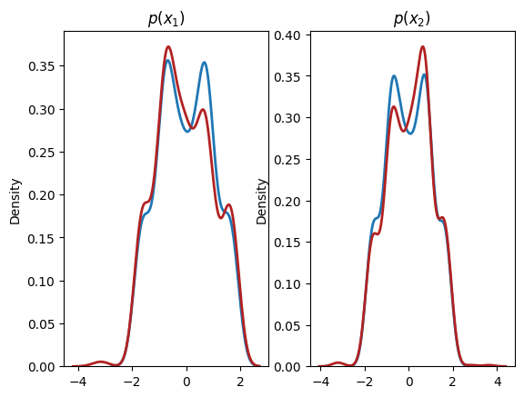

which from the plot, seems close to the actual distribution. Of course, we can do even better but that’s for later.

There are several other libraries available for using the Normalizing Flows method such as normflows , ProbFlow, etc. In addition, I found the following resources to be helpful:

1. https://gowrishankar.info/blog/normalizing-flows-a-practical-guide-using-tensorflow-probability/
2. https://github.com/LukasRinder/normalizing-flows
3. https://probflow.readthedocs.io/en/latest/examples/normalizing_flows.html
4. https://github.com/VincentStimper/normalizing-flows
5. https://github.com/tatsy/normalizing-flows-pytorch
6. https://vishakh.me/posts/normalizing_flows/
7. https://uvadlc-notebooks.readthedocs.io/en/latest/tutorial_notebooks/tutorial11/NF_image_modeling.html
8. https://gebob19.github.io/normalizing-flows/

Conclusion

The article provides a concise introduction to the Normalizing Flows method starting from the variable transformation to generating new distribution. The application of this statistical method combined with the neural network ranges from fake image generation to anomaly detection and finding novel molecules and materials. I recommend readers check the resources I mentioned above to get a deeper understanding of the Normalizing Flows. In future articles, I will present new developments in Normalizing Flows.

The notebook associated with the Python code above can be obtained here: https://github.com/rahulbhadani/medium.com/blob/ec92a9bc7b2aa165df630ed5e268ec58fc0716a2/10_09_2022/normflow.ipynb

References

1. Clustering and classification through normalizing flows in feature space https://www.researchgate.net/profile/Martin-Cadeiras/publication/220385824_Clustering_and_Classification_through_Normalizing_Flows_in_Feature_Space/links/54da12330cf2464758204dbb/Clustering-and-Classification-through-Normalizing-Flows-in-Feature-Space.pdf
2. A family of non-parametric density estimation algorithms https://ri.conicet.gov.ar/bitstream/handle/11336/8930/CONICET_Digital_Nro.12124.pdf?sequence=1
3. Kobyzev, I., Prince, S. J., & Brubaker, M. A. (2020). Normalizing flows: An introduction and review of current methods. IEEE transactions on pattern analysis and machine intelligence, 43(11), 3964–3979.

I hope this article was helpful to you in getting started with an exciting topic in statistics and data science.

Was this helpful? Buy me a Coffee.

Love my writing? Join my email list.

Want to know more about STEM-related topics? Join Medium.