
Speech Recognition — Feature Extraction MFCC & PLP

Machine learning ML extracts features from raw data and creates a dense representation of the content. This forces us to learn the core information without the noise to make inferences (if it is done correctly).
Back to the speech recognition, our objective is finding the best sequence of words corresponding to the audio based on the acoustic and language model.

To create an acoustic model, our observation X is represented by a sequence of acoustic feature vectors (x₁, x₂, x₃, …). In the previous article, we learn how people articulate and perceive speech. In this article, we discuss how audio features are extracted from what we learned.
Requirement
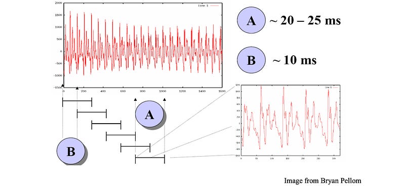
Let’s define some of the requirements for the feature extraction in ASR (Automatic speech recognizer) first. Given an audio segment, we are using a sliding window of 25ms wide to extract audio features.
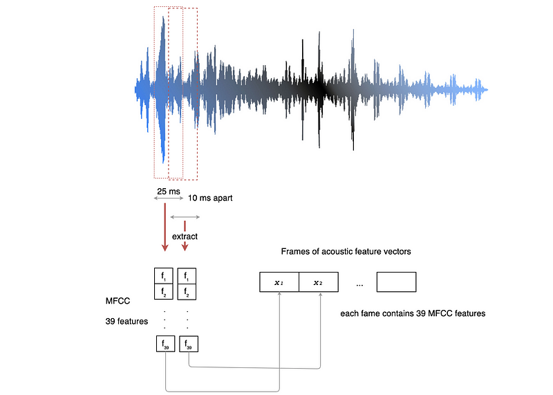
This 25ms width is large enough for us to capture enough information and yet the features inside this frame should remain relatively stationary. If we speak 3 words per second with 4 phones and each phone will be sub-divided into 3 stages, then there are 36 states per second or 28 ms per state. So the 25ms window is about right.
Context is very important in speech. Pronunciations are changed according to the articulation before and after a phone. Each slid window is about 10ms apart so we can capture the dynamics among frames to capture the proper context.
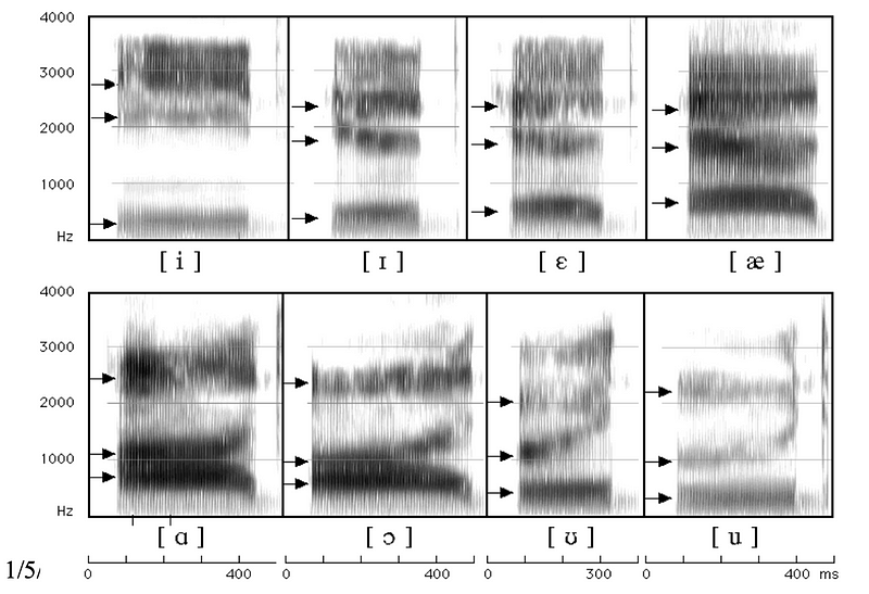
Pitch varies with people. However, this has little role in recognizing what he/she said. F0 is related to the pitch. It provides no value in speech recognition and should be removed. What is more important is the formants F1, F2, F3, … For those that have problems in following these terms, we suggest you read the previous article first.
We also hope the extracted features will be robust to who the speaker is, and the noise in the environments. Also, like any ML problems, we want extracted features to be independent of others. It is easier to develop models and to train these models with independent features.
One popular audio feature extraction method is the Mel-frequency cepstral coefficients (MFCC) which have 39 features. The feature count is small enough to force us to learn the information of the audio. 12 parameters are related to the amplitude of frequencies. It provides us enough frequency channels to analyze the audio.
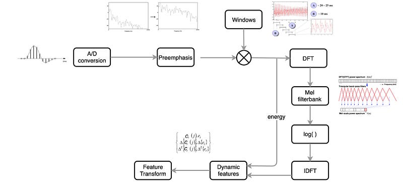
Below is the flow of extracting the MFCC features.
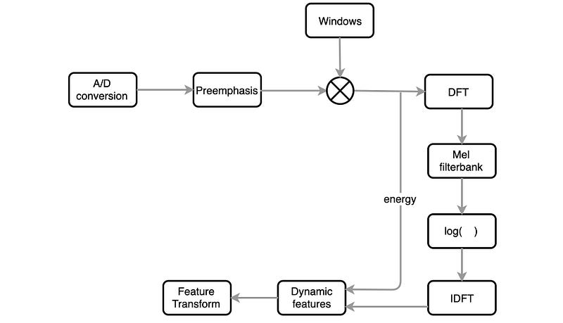
The key objectives are:
- Remove vocal fold excitation (F0) — the pitch information.
- Make the extracted features independent.
- Adjust to how humans perceive loudness and frequency of sound.
- Capture the dynamics of phones (the context).
Mel-frequency cepstral coefficients (MFCC)
Let’s cover each step one at a time.
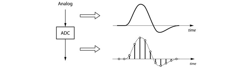
A/D conversion
A/D conversion samples the audio clips and digitizes the content, i.e. converting the analog signal into discrete space. A sampling frequency of 8 or 16 kHz is often used.
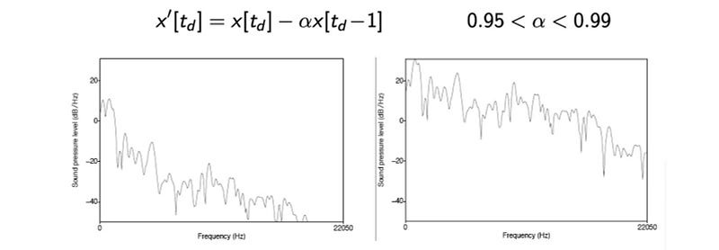
Pre-emphasis
Pre-emphasis boosts the amount of energy in the high frequencies. For voiced segments like vowels, there is more energy at the lower frequencies than the higher frequencies. This is called spectral tilt which is related to the glottal source (how vocal folds produce sound). Boosting the high-frequency energy makes information in higher formants more available to the acoustic model. This improves phone detection accuracy. For humans, we start having hearing problems when we cannot hear these high-frequency sounds. Also, noise has a high frequency. In the engineering field, we use pre-emphasis to make the system less susceptible to noise introduced in the process later. For some applications, we just need to undo the boosting at the end.
Pre-emphasis uses a filter to boost higher frequencies. Below is the before and after signal on how the high-frequency signal is boosted.
Windowing
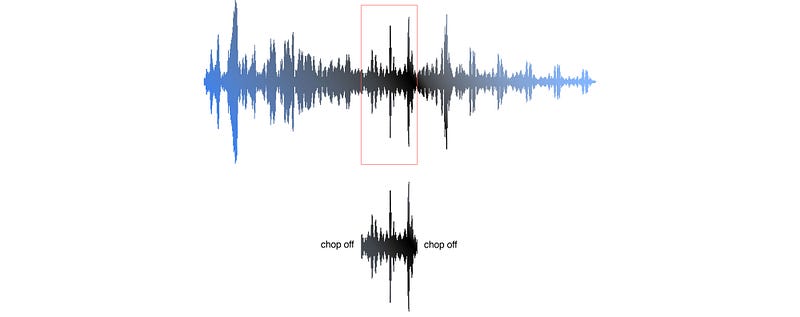
Windowing involves the slicing of the audio waveform into sliding frames.
But we cannot just chop it off at the edge of the frame. The suddenly fallen in amplitude will create a lot of noise that shows up in the high-frequency. To slice the audio, the amplitude should gradually drop off near the edge of a frame.
Let’s say w is the window applied to the original audio clip in the time domain.

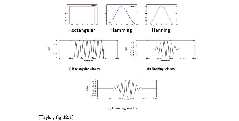
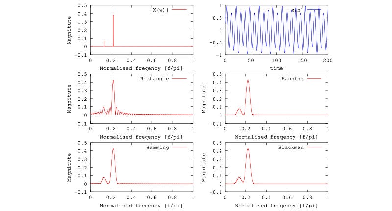
A few alternatives for w are the Hamming window and the Hanning window. The following diagram indicates how a sinusoidal waveform will be chopped off using these windows. As shown, for Hamming and Hanning window, the amplitude drops off near the edge. (The Hamming window has a slight sudden drop at the edge while the Hanning window does not.)
The corresponding equations for w are:

On the top right below is a soundwave in the time domain. It mainly composes of two frequencies only. As shown, the chopped frame with Hamming and Hanning maintains the original frequency information better with less noise compared to a rectangle window.
Discrete Fourier Transform (DFT)
Next, we apply DFT to extract information in the frequency domain.

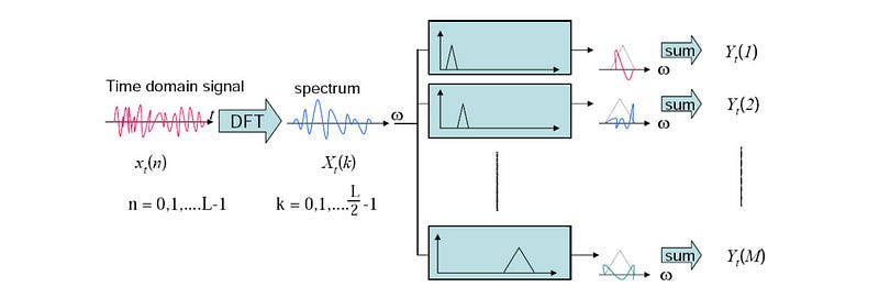
Mel filterbank
As mentioned in the previous article, the equipment measurements are not the same as our hearing perception. For humans, the perceived loudness changes according to frequency. Also, perceived frequency resolution decreases as frequency increases. i.e. humans are less sensitive to higher frequencies. The diagram on the left indicates how the Mel scale maps the measured frequency to that we perceived in the context of frequency resolution.
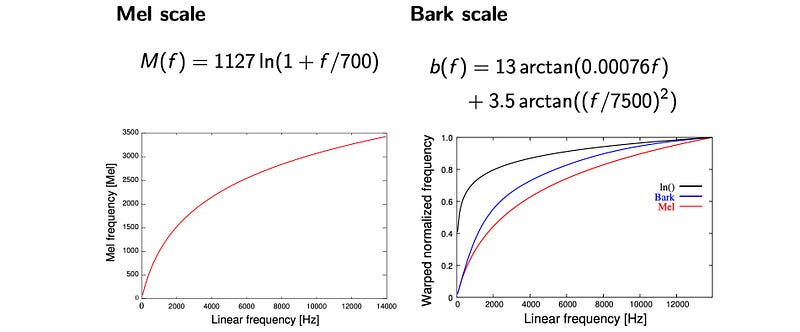
All these mappings are non-linear. In feature extraction, we apply triangular band-pass filters to coverts the frequency information to mimic what a human perceived.
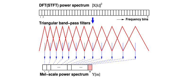
First, we square the output of the DFT. This reflects the power of the speech at each frequency (x[k]²) and we call it the DFT power spectrum. We apply these triangular Mel-scale filter banks to transform it to Mel-scale power spectrum. The output for each Mel-scale power spectrum slot represents the energy from a number of frequency bands that it covers. This mapping is called the Mel Binning. The precise equations for slot m will be:

The Trainangular bandpass is wider at the higher frequencies to reflect human hearing is less sensitivity in high frequency. Specifically, it is linearly spaced below 1000 Hz and turns logarithmically afterward.
All these efforts try to mimic how the basilar membrane in our ear senses the vibration of sounds. The basilar membrane has about 15,000 hairs inside the cochlear at birth. The diagram below demonstrates the frequency response of those hairs. So the curve-shape response below is simply approximated by triangles in Mel filterbank.
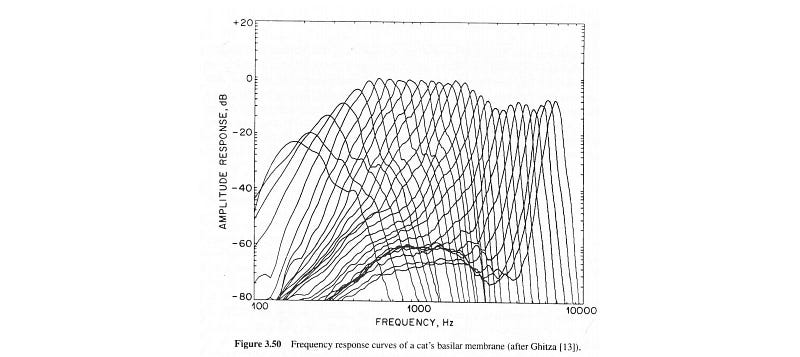
We imitate how our ears perceive sound through those hairs. In short, it is modeled by the triangular filters using Mel filtering bank.
Log
Mel filterbank outputs a power spectrum. Humans are less sensitive to small energy change at high energy than small changes at a low energy level. In fact, it is logarithmic. So our next step will take the log out of the output of the Mel filterbank. This also reduces the acoustic variants that are not significant for speech recognition. Next, we need to address two more requirements. First, we need to remove the F0 information (the pitch) and makes the extracted features independent of others.
Cepstrum — IDFT
Below is the model of how speech is produced.
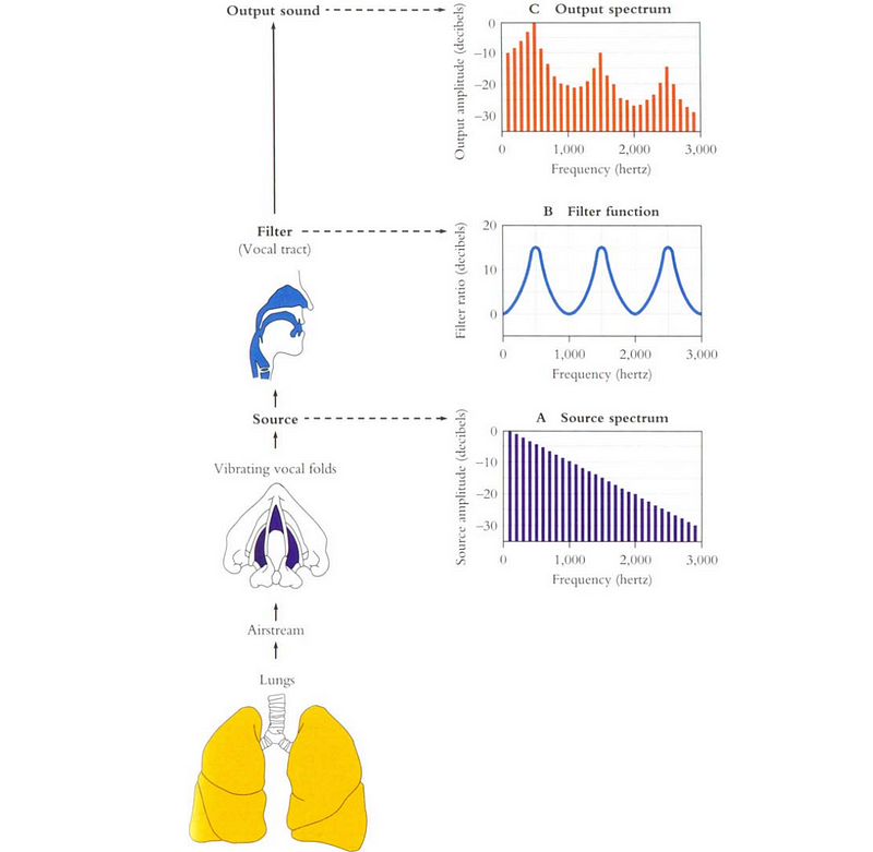
Our articulations control the shape of the vocal tract. The source-filter model combines the vibrations produced by the vocal folds with the filter created by our articulations. The glottal source waveform will be suppressed or amplified at different frequencies by the shape of the vocal tract.
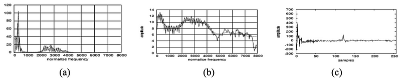
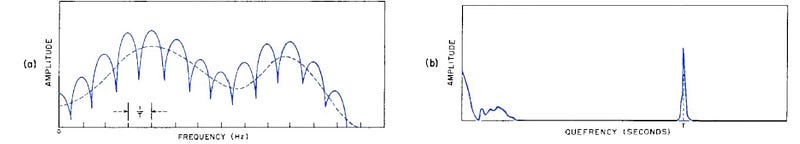
Cepstrum is the reverse of the first 4 letters in the word “spectrum”. Our next step is to compute the Cepstral which separates the glottal source and the filter. Diagram (a) is the spectrum with the y-axis being the magnitude. Diagram (b) takes the log of the magnitude. Look closer, the wave fluctuates about 8 times between 1000 and 2000. Actually, it fluctuates about 8 times for every 1000 units. That is about 125 Hz — the source vibration of the vocal folds.
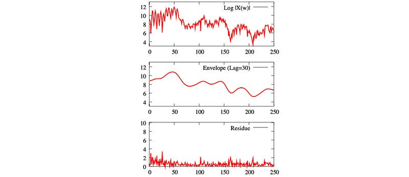
As observed, the log spectrum (the first diagram below) composes of information related to the phone (the second diagram) and the pitch (the third diagram). The peaks in the second diagram identify the formants that distinguish phones. But how can we separate them?
Recall that periods in the time or frequency domain is inverted after transformation.
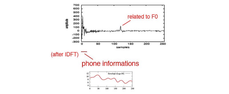
Recall that the pitch information has short periods in the frequency domain. We can apply the inverse Fourier Transformation to separate the pitch information from the formants. As shown below, the pitch information will show up on the middle and the right side. The peak in the middle is actually corresponding to F0 and the phone-related information will locate in the far left.
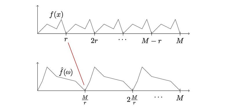
Here is another visualization. The solid line on the left diagram is the signal in the frequency domain. It is composed of the phone information drawn in the dotted line and the pitch information. After the IDFT (inverse Discrete Fourier Transform), the pitch information with 1/T period is transformed to a peak near T at the right side.
So for speech recognition, we just need the coefficients on the far left and discard the others. In fact, MFCC just takes the first 12 cepstral values. There is another important property related to these 12 coefficients. Log power spectrum is real and symmetric. Its inverse DFT is equivalent to a discrete cosine transformation (DCT).

DCT is an orthogonal transformation. Mathematically, the transformation produces uncorrelated features. Therefore, MFCC features are highly unrelated. In ML, this makes our model easier to model and to train. If we model these parameters with multivariate Gaussian distribution, all the non-diagonal values in the covariance matrix will be zero. Mathematically, the output of this stage is

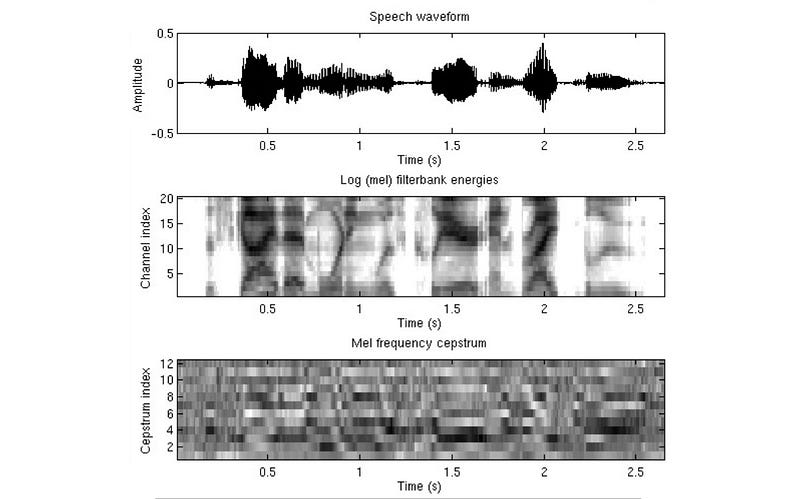
The following is the visualization of the 12 Cepstrum coefficients.
Dynamic features (delta)
MFCC has 39 features. We finalize 12 and what are the rest. The 13th parameter is the energy in each frame. It helps us to identify phones.

In pronunciation, context and dynamic information are important. Articulations, like stop closures and releases, can be recognized by the formant transitions. Characterizing feature changes over time provides the context information for a phone. Another 13 values compute the delta values d(t) below. It measures the changes in features from the previous frame to the next frame. This is the first-order derivative of the features.

The last 13 parameters are the dynamic changes of d(t) from the last frame to the next frame. It acts as the second-order derivative of c(t).
So the 39 MFCC features parameters are 12 Cepstrum coefficients plus the energy term. Then we have 2 more sets corresponding to the delta and the double delta values.
Cepstral mean and variance normalization
Next, we can perform the feature normalization. We normalize the features with its mean and divide it by its variance. The mean and variance are computed with the feature value j over all the frames in a single utterance. This allows us to adjust values to countermeasure the variants in each recording.

However, if the audio clip is short, this may not be reliable. Instead, we may compute the average and variance values based on speakers, or even over the entire training dataset. This type of feature normalization will effectively cancel the pre-emphasis done earlier. That is how we extract MFCC features. As a last note, MFCC is not very robust against noise.
Perceptual Linear Prediction (PLP)
PLP is very similar to MFCC. Motivated by hearing perception, it uses equal loudness pre-emphasis and cube-root compression instead of the log compression.
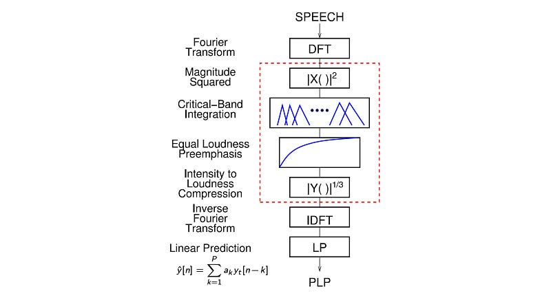
It also uses linear regressive to finalize the cepstral coefficients. PLP has slightly better accuracy and slightly better noise robustness. But it is also believed that MFCC is a safe choice. Throughout this series, when we say we extract MFCC features, we can extract PLP features instead also.
Thoughts
ML builds a model for the problem domain. For complex problems, this is extremely hard and the approach is usually very heuristic. Sometimes, people think we are hacking the system. The feature extraction methods in this article depend strongly on empirical results and observations. With the introduction of DL, we can train complex models with less hacking. However, some of the concepts remain valid and important for DL speech recognition.
Next
To go deeper into speech recognition, we need to study two ML algorithms in details.


