

Softmax Classifier using TensorFlow on MNIST dataset with sample code
install tensorflow
!pip install tensorflowLoading Mnist dataset
Every MNIST data point has two parts: an image of a handwritten digit and a corresponding label. We’ll call the images “x” and the labels “y”. Both the training set and test set contain images and their corresponding labels; for example the training images are mnist.train.images and the training labels are mnist.train.labels.
import tensorflow.examples.tutorials.mnist.input_data as input_data
mnist=input_data.read_data_sets(“MNIST”, one_hot=True)
Check dimension of train and test of MNIST dataset
print(“number of data points : “, mnist.train.images.shape[0],”number of pixels in each image :”,mnist.train.images.shape[1])Number of train data points : 55000 number of pixels in each image : 784
mnist.train.images is a tensor (an n-dimensional array) with a shape of [55000, 784]. The first dimension is an index into the list of images and the second dimension is the index for each pixel in each image. Each entry in the tensor is a pixel intensity between 0 and 1, for a particular pixel in a particular image.
print(“number of data points : “, mnist.test.labels.shape[0],” length of the one hot encoded label vector :”,mnist.test.labels.shape[1])Number of test data points: 10000 length of the one hot encoded label vector : 10
Activate library
If you want to assign probabilities to an object being one of several different things, softmax (Multiclass Logistic regression) is the thing to do, because softmax gives us a list of values between 0 and 1 that add up to 1. Even later on, when we train more sophisticated models, the final step will be a layer of softmax.
import tensorflow as tf
import numpy as np
Defining Placeholders, Variables, predicted y and loss function
x = tf.placeholder(tf.float32, [None, 784])x isn’t a specific value. It’s a placeholder. A placeholder can be imagined as a memory unit that we use to load various mini-batches of input data while training. We want to be able to input any number of MNIST images, each flattened into a 784-dimensional vector. We represent this as a 2-D tensor of floating-point numbers, with a shape [None, 784] (Here None means that a dimension can be of any length.)
W = tf.Variable(tf.zeros([784, 10]))
b = tf.Variable(tf.zeros([10]))
We also need the weights and biases for our model. We could imagine treating these like additional inputs, but TensorFlow has an even better way to handle it: Variable.
y = tf.nn.softmax(tf.matmul(x, W) + b)# predicted y
y_ = tf.placeholder(tf.float32, [None, 10])#actual y
Now, First, we multiply x by W with the expression tf.matmul(x, W). This is flipped from when we multiplied them in our equation, where we had Wx, as a small trick to deal with x being a 2D tensor with multiple inputs. We then add b, and finally apply tf.nn.softmax.
cross_entropy = tf.reduce_mean(-tf.reduce_sum(y_ * tf.log(y), reduction_indices=[1]))#Tutorial for tf.reduce_sum: https://www.dotnetperls.com/reduce-sum-tensorflowDefining the loss function: multi-class log-loss/cross-entropy First, tf.log computes the logarithm of each element of y. Next, we multiply each element of y_ with the corresponding element of tf.log(y). Then tf.reduce_sum adds the elements in the second dimension of y, due to the reduction_indices=[1] parameter. Finally, tf.reduce_mean computes the mean over all the examples in the batch. Reduction is an operation that removes one or more dimensions from a tensor by performing certain operations across those dimensions.
Defining optimizer
train_step=tf.train.GradientDescentOptimizer(0.05).minimize(cross_entropy)
#https://www.tensorflow.org/versions/r1.2/api_guides/python/train#Optimizers
In this case, we ask TensorFlow to minimize cross_entropy using the gradient descent algorithm with a learning rate of 0.05. What TensorFlow actually does here, behind the scenes, is to add new operations to your computation-graph which implement backpropagation and gradient descent. Then it gives you back a single operation which, when run, does a step of gradient descent training, slightly tweaking your variables to reduce the loss.
Launch model
#Now launch the model in an InteractiveSession
sess = tf.InteractiveSession()
We first have to create an operation to initialize the variables we created:
tf.global_variables_initializer().run()# We run train_step feeding in the batches data to replace the placeholders
for _ in range(1000):
 batch_xs, batch_ys = mnist.train.next_batch(100)
 sess.run(train_step, feed_dict={x: batch_xs, y_: batch_ys})
Each step of the loop, we get a “mini-batch” of one hundred random data points from our training set. Using small batches of random data is called stochastic training — in this case, stochastic gradient descent. Ideally, we’d like to use all our data for every step of training because that would give us a better sense of what we should be doing, but that’s expensive. So, instead, we use a different subset every time. Doing this is cheap and has much of the same benefit.
# https://stackoverflow.com/a/41863099

correct_prediction = tf.equal(tf.argmax(y,1), tf.argmax(y_,1))
accuracy = tf.reduce_mean(tf.cast(correct_prediction, tf.float32))
print(sess.run(accuracy, feed_dict={x: mnist.test.images, y_: mnist.test.labels}))
tf.argmax(input, axis=None, name=None, dimension=None) Returns the index with the largest value across axis of a tensor.
Plotting error
# https://gist.github.com/greydanus/f6eee59eaf1d90fcb3b534a25362cea4
# https://stackoverflow.com/a/14434334
%matplotlib notebook
import matplotlib.pyplot as plt
import numpy as np
import time

def plt_dynamic(x, y, y_1, ax, colors=[‘b’]):
   ax.plot(x, y, ‘b’, label=”Train Loss”)
   ax.plot(x, y_1, ‘r’, label=”Test Loss”)
   if len(x)==1:
   plt.legend()
   fig.canvas.draw()
Now summarizing everything in a single cell
training_epochs = 15
batch_size = 1000
display_step = 1
cross_entropy = tf.reduce_mean(tf.nn.softmax_cross_entropy_with_logits(logits = y, labels = y_))
train_step = tf.train.GradientDescentOptimizer(0.05).minimize(cross_entropy)
fig,ax = plt.subplots(1,1)
ax.set_xlabel(‘epoch’) ; ax.set_ylabel(‘Soft Max Cross Entropy loss’)
xs, ytrs, ytes = [], [], []
for epoch in range(training_epochs):
train_avg_cost = 0.
test_avg_cost = 0.
total_batch = int(mnist.train.num_examples/batch_size)
# Loop over all batches
for i in range(total_batch):
batch_xs, batch_ys = mnist.train.next_batch(batch_size)
_, c = sess.run([train_step, cross_entropy], feed_dict={x: batch_xs, y_: batch_ys})
train_avg_cost += c / total_batch
c = sess.run(cross_entropy, feed_dict={x: mnist.test.images, y_: mnist.test.labels})
test_avg_cost += c / total_batchxs.append(epoch)
ytrs.append(train_avg_cost)
ytes.append(test_avg_cost)
plt_dynamic(xs, ytrs, ytes, ax)plt_dynamic(xs, ytrs, ytes, ax)
correct_prediction = tf.equal(tf.argmax(y,1), tf.argmax(y_,1))
accuracy = tf.reduce_mean(tf.cast(correct_prediction, tf.float32))
print(“Accuracy:”, accuracy.eval({x: mnist.test.images, y_: mnist.test.labels}))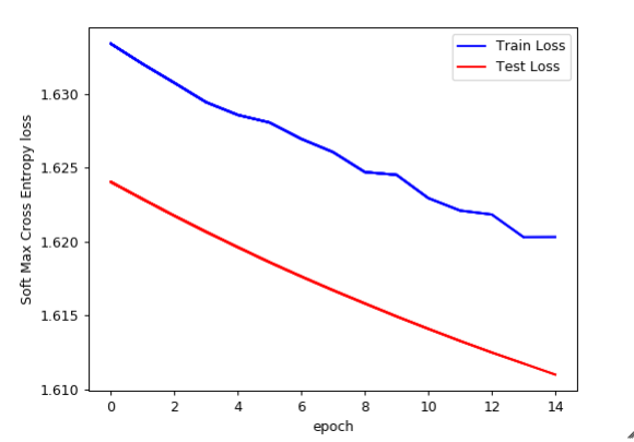
Above plot is between log-loss vs number of epochs where the blue line show train error and red line show the test error.
Accuracy obtains using tensor flow is 90% on MNIST dataset.
=====Detail code can be found at below GitHub link =======
Reference:
- Applied AI(special thanks)
- https://www.tensorflow.org/
- Google image
======================================


