Simple Reinforcement Learning with Tensorflow Part 8: Asynchronous Actor-Critic Agents (A3C)

In this article I want to provide a tutorial on implementing the Asynchronous Advantage Actor-Critic (A3C) algorithm in Tensorflow. We will use it to solve a simple challenge in a 3D Doom environment! With the holidays right around the corner, this will be my final post for the year, and I hope it will serve as a culmination of all the previous topics in the series. If you haven’t yet, or are new to Deep Learning and Reinforcement Learning, I suggest checking out the earlier entries in the series before going through this post in order to understand all the building blocks which will be utilized here. If you have been following the series: thank you! I have learned so much about RL in the past year, and am happy to have shared it with everyone through this article series.

So what is A3C? The A3C algorithm was released by Google’s DeepMind group earlier this year, and it made a splash by… essentially obsoleting DQN. It was faster, simpler, more robust, and able to achieve much better scores on the standard battery of Deep RL tasks. On top of all that it could work in continuous as well as discrete action spaces. Given this, it has become the go-to Deep RL algorithm for new challenging problems with complex state and action spaces. In fact, OpenAI just released a version of A3C as their “universal starter agent” for working with their new (and very diverse) set of Universe environments.

The 3 As of A3C

Asynchronous Advantage Actor-Critic is quite a mouthful. Let’s start by unpacking the name, and from there, begin to unpack the mechanics of the algorithm itself.

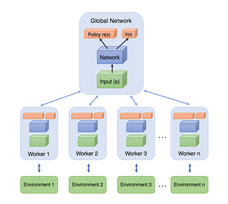
Asynchronous: Unlike DQN, where a single agent represented by a single neural network interacts with a single environment, A3C utilizes multiple incarnations of the above in order to learn more efficiently. In A3C there is a global network, and multiple worker agents which each have their own set of network parameters. Each of these agents interacts with it’s own copy of the environment at the same time as the other agents are interacting with their environments. The reason this works better than having a single agent (beyond the speedup of getting more work done), is that the experience of each agent is independent of the experience of the others. In this way the overall experience available for training becomes more diverse.

Actor-Critic: So far this series has focused on value-iteration methods such as Q-learning, or policy-iteration methods such as Policy Gradient. Actor-Critic combines the benefits of both approaches. In the case of A3C, our network will estimate both a value function V(s) (how good a certain state is to be in) and a policy π(s) (a set of action probability outputs). These will each be separate fully-connected layers sitting at the top of the network. Critically, the agent uses the value estimate (the critic) to update the policy (the actor) more intelligently than traditional policy gradient methods.

Advantage: If we think back to our implementation of Policy Gradient, the update rule used the discounted returns from a set of experiences in order to tell the agent which of its actions were “good” and which were “bad.” The network was then updated in order to encourage and discourage actions appropriately.

Discounted Reward: R = γ(r)

The insight of using advantage estimates rather than just discounted returns is to allow the agent to determine not just how good its actions were, but how much better they turned out to be than expected. Intuitively, this allows the algorithm to focus on where the network’s predictions were lacking. If you recall from the Dueling Q-Network architecture, the advantage function is as follow:

Advantage: A = Q(s,a) - V(s)

Since we won’t be determining the Q values directly in A3C, we can use the discounted returns (R) as an estimate of Q(s,a) to allow us to generate an estimate of the advantage.

Advantage Estimate: A = R - V(s)

In this tutorial, we will go even further, and utilize a slightly different version of advantage estimation with lower variance referred to as Generalized Advantage Estimation.

Implementing the Algorithm

Training workflow of each worker agent in A3C.

In the process of building this implementation of the A3C algorithm, I used as reference the quality implementations by DennyBritz and OpenAI. Both of which I highly recommend if you’d like to see alternatives to my code here. Each section embedded here is taken out of context for instructional purposes, and won’t run on its own. To view and run the full, functional A3C implementation, see my Github repository.

The general outline of the code architecture is:

AC_Network — This class contains all the Tensorflow ops to create the networks themselves.
Worker — This class contains a copy of AC_Network, an environment class, as well as all the logic for interacting with the environment, and updating the global network.
High-level code for establishing the Worker instances and running them in parallel.

The A3C algorithm begins by constructing the global network. This network will consist of convolutional layers to process spatial dependencies, followed by an LSTM layer to process temporal dependencies, and finally, value and policy output layers. Below is example code for establishing the network graph itself.

Next, a set of worker agents, each with their own network and environment are created. Each of these workers are run on a separate processor thread, so there should be no more workers than there are threads on your CPU.

~ From here we go asynchronous ~

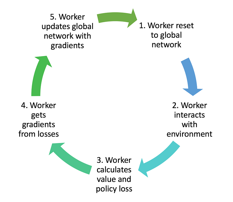
Each worker begins by setting its network parameters to those of the global network. We can do this by constructing a Tensorflow op which sets each variable in the local worker network to the equivalent variable value in the global network.

Each worker then interacts with its own copy of the environment and collects experience. Each keeps a list of experience tuples (observation, action, reward, done, value) that is constantly added to from interactions with the environment.

Once the worker’s experience history is large enough, we use it to determine discounted return and advantage, and use those to calculate value and policy losses. We also calculate an entropy (H) of the policy. This corresponds to the spread of action probabilities. If the policy outputs actions with relatively similar probabilities, then entropy will be high, but if the policy suggests a single action with a large probability then entropy will be low. We use the entropy as a means of improving exploration, by encouraging the model to be conservative regarding its sureness of the correct action.

Value Loss: L = Σ(R - V(s))²

Policy Loss: L = -log(π(s)) * A(s) - β*H(π)

A worker then uses these losses to obtain gradients with respect to its network parameters. Each of these gradients are typically clipped in order to prevent overly-large parameter updates which can destabilize the policy.

A worker then uses the gradients to update the global network parameters. In this way, the global network is constantly being updated by each of the agents, as they interact with their environment.

Once a successful update is made to the global network, the whole process repeats! The worker then resets its own network parameters to those of the global network, and the process begins again.

To view the full and functional code, see the Github repository here.

Playing Doom

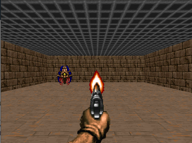
The robustness of A3C allows us to tackle a new generation of reinforcement learning challenges, one of which is 3D environments! We have come a long way from multi-armed bandits and grid-worlds, and in this tutorial, I have set up the code to allow for playing through the first VizDoom challenge. VizDoom is a system to allow for RL research using the classic Doom game engine. The maintainers of VizDoom recently created a pip package, so installing it is as simple as:

pip install vizdoom

Once it is installed, we will be using the basic.wad environment, which is provided in the Github repository, and needs to be placed in the working directory.

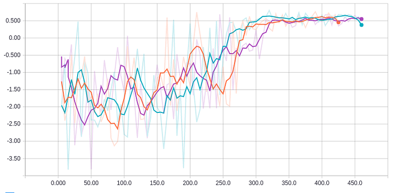
The challenge consists of controlling an avatar from a first person perspective in a single square room. There is a single enemy on the opposite side of the room, which appears in a random location each episode. The agent can only move to the left or right, and fire a gun. The goal is to shoot the enemy as quickly as possible using as few bullets as possible. The agent has 300 time steps per episode to shoot the enemy. Shooting the enemy yields a reward of 1, and each time step as well as each shot yields a small penalty. After about 500 episodes per worker agent, the network learns a policy to quickly solve the challenge. Feel free to adjust parameters such as learning rate, clipping magnitude, update frequency, etc. to attempt to achieve ever greater performance or utilize A3C in your own RL tasks.

Average reward over time for three workers on Doom task. 0.5 reward corresponds to optimal performance. X-axis represents number of training episodes per worker.

I hope this tutorial has been helpful to those new to A3C and asynchronous reinforcement learning! Now go forth and build AIs.

(There are a lot of moving parts in A3C, so if you discover a bug, or find a better way to do something, please don’t hesitate to bring it up here or in the Github. I am more than happy to incorporate changes and feedback to improve the algorithm.)

If you’d like to follow my writing on Deep Learning, AI, and Cognitive Science, follow me on Medium @Arthur Juliani, or on twitter @awjuliani.

If this post has been valuable to you, please consider donating to help support future tutorials, articles, and implementations. Any contribution is greatly appreciated!

More from my Simple Reinforcement Learning with Tensorflow series: