
Simple and Multiple Linear Regression in Python
Quick introduction to linear regression in Python
Hi everyone! After briefly introducing the “Pandas” library as well as the NumPy library, I wanted to provide a quick introduction to building models in Python, and what better place to start than one of the very basic models, linear regression? This will be the first post about machine learning and I plan to write about more complex models in the future. Stay tuned! But for right now, let’s focus on linear regression.
In this blog post, I want to focus on the concept of linear regression and mainly on the implementation of it in Python. Linear regression is a statistical model that examines the linear relationship between two (Simple Linear Regression ) or more (Multiple Linear Regression) variables — a dependent variable and independent variable(s). Linear relationship basically means that when one (or more) independent variables increases (or decreases), the dependent variable increases (or decreases) too:
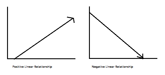
As you can see, a linear relationship can be positive (independent variable goes up, dependent variable goes up) or negative (independent variable goes up, dependent variable goes down). Like I said, I will focus on the implementation of regression models in Python, so I don’t want to delve too much into the math under the regression hood, but I will write a little bit about it. If you’d like a blog post about that, please don’t hesitate to write me in the responses!
A Little Bit About the Math
A relationship between variables Y and X is represented by this equation:
Y`i = mX + b
In this equation, Y is the dependent variable — or the variable we are trying to predict or estimate; X is the independent variable — the variable we are using to make predictions; m is the slope of the regression line — it represent the effect X has on Y. In other words, if X increases by 1 unit, Y will increase by exactly m units. (“Full disclosure”: this is true only if we know that X and Y have a linear relationship. In almost all linear regression cases, this will not be true!) b is a constant, also known as the Y-intercept. If X equals 0, Y would be equal to b (Caveat: see full disclosure from earlier!). This is not necessarily applicable in real life — we won’t always know the exact relationship between X and Y or have an exact linear relationship.
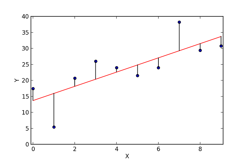
These caveats lead us to a Simple Linear Regression (SLR). In a SLR model, we build a model based on data — the slope and Y-intercept derive from the data; furthermore, we don’t need the relationship between X and Y to be exactly linear. SLR models also include the errors in the data (also known as residuals). I won’t go too much into it now, maybe in a later post, but residuals are basically the differences between the true value of Y and the predicted/estimated value of Y. It is important to note that in a linear regression, we are trying to predict a continuous variable. In a regression model, we are trying to minimize these errors by finding the “line of best fit” — the regression line from the errors would be minimal. We are trying to minimize the length of the black lines (or more accurately, the distance of the blue dots) from the red line — as close to zero as possible. It is related to (or equivalent to) minimizing the mean squared error (MSE) or the sum of squares of error (SSE), also called the “residual sum of squares.” (RSS) but this might be beyond the scope of this blog post :-)
In most cases, we will have more than one independent variable — we’ll have multiple variables; it can be as little as two independent variables and up to hundreds (or theoretically even thousands) of variables. in those cases we will use a Multiple Linear Regression model (MLR). The regression equation is pretty much the same as the simple regression equation, just with more variables:
Y’i = b0 + b1X1i + b2X2iThis concludes the math portion of this post :) Ready to get to implementing it in Python?
Linear Regression in Python
There are two main ways to perform linear regression in Python — with Statsmodels and scikit-learn. It is also possible to use the Scipy library, but I feel this is not as common as the two other libraries I’ve mentioned. Let’s look into doing linear regression in both of them:
Linear Regression in Statsmodels
Statsmodels is “a Python module that provides classes and functions for the estimation of many different statistical models, as well as for conducting statistical tests, and statistical data exploration.” (from the documentation)
As in with Pandas and NumPy, the easiest way to get or install Statsmodels is through the Anaconda package. If, for some reason you are interested in installing in another way, check out this link. After installing it, you will need to import it every time you want to use it:
import statsmodels.api as smLet’s see how to actually use Statsmodels for linear regression. I’ll use an example from the data science class I took at General Assembly DC:
First, we import a dataset from sklearn (the other library I’ve mentioned):
from sklearn import datasets ## imports datasets from scikit-learn
data = datasets.load_boston() ## loads Boston dataset from datasets library
This is a dataset of the Boston house prices (link to the description). Because it is a dataset designated for testing and learning machine learning tools, it comes with a description of the dataset, and we can see it by using the command print data.DESCR (this is only true for sklearn datasets, not every dataset! Would have been cool though…). I’m adding the beginning of the description, for better understanding of the variables:
Boston House Prices dataset
===========================

Notes
------
Data Set Characteristics:

    :Number of Instances: 506

    :Number of Attributes: 13 numeric/categorical predictive

    :Median Value (attribute 14) is usually the target

    :Attribute Information (in order):
        - CRIM     per capita crime rate by town
        - ZN       proportion of residential land zoned for lots over 25,000 sq.ft.
        - INDUS    proportion of non-retail business acres per town
        - CHAS     Charles River dummy variable (= 1 if tract bounds river; 0 otherwise)
        - NOX      nitric oxides concentration (parts per 10 million)
        - RM       average number of rooms per dwelling
        - AGE      proportion of owner-occupied units built prior to 1940
        - DIS      weighted distances to five Boston employment centres
        - RAD      index of accessibility to radial highways
        - TAX      full-value property-tax rate per $10,000
        - PTRATIO  pupil-teacher ratio by town
        - B        1000(Bk - 0.63)^2 where Bk is the proportion of blacks by town
        - LSTAT    % lower status of the population
        - MEDV     Median value of owner-occupied homes in $1000's

    :Missing Attribute Values: None

    :Creator: Harrison, D. and Rubinfeld, D.L.

This is a copy of UCI ML housing dataset.
http://archive.ics.uci.edu/ml/datasets/Housing


This dataset was taken from the StatLib library which is maintained at Carnegie Mellon University.
Running data.feature_names and data.target would print the column names of the independent variables and the dependent variable, respectively. Meaning, Scikit-learn has already set the house value/price data as a target variable and 13 other variables are set as predictors. Let’s see how to run a linear regression on this dataset.
First, we should load the data as a pandas data frame for easier analysis and set the median home value as our target variable:
import numpy as np
import pandas as pd
# define the data/predictors as the pre-set feature names
df = pd.DataFrame(data.data, columns=data.feature_names)
# Put the target (housing value -- MEDV) in another DataFrame
target = pd.DataFrame(data.target, columns=["MEDV"])What we’ve done here is to take the dataset and load it as a pandas data frame; after that, we’re setting the predictors (as df) — the independent variables that are pre-set in the dataset. We’re also setting the target — the dependent variable, or the variable we’re trying to predict/estimate.
Next we’ll want to fit a linear regression model. We need to choose variables that we think we’ll be good predictors for the dependent variable — that can be done by checking the correlation(s) between variables, by plotting the data and searching visually for relationship, by conducting preliminary research on what variables are good predictors of y etc. For this first example, let’s take RM — the average number of rooms and LSTAT — percentage of lower status of the population. It’s important to note that Statsmodels does not add a constant by default. Let’s see it first without a constant in our regression model:
## Without a constant
import statsmodels.api as sm
X = df["RM"]
y = target["MEDV"]
# Note the difference in argument order
model = sm.OLS(y, X).fit()
predictions = model.predict(X) # make the predictions by the model
# Print out the statistics
model.summary()The output:
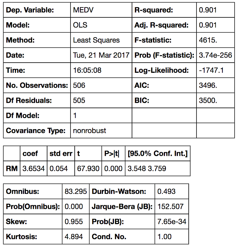
Interpreting the Table —This is a very long table, isn’t it? First we have what’s the dependent variable and the model and the method. OLS stands for Ordinary Least Squares and the method “Least Squares” means that we’re trying to fit a regression line that would minimize the square of distance from the regression line (see the previous section of this post). Date and Time are pretty self-explanatory :) So as number of observations. Df of residuals and models relates to the degrees of freedom — “the number of values in the final calculation of a statistic that are free to vary.”
The coefficient of 3.6534 means that as the RM variable increases by 1, the predicted value of MDEV increases by 3.6534. A few other important values are the R-squared — the percentage of variance our model explains; the standard error (is the standard deviation of the sampling distribution of a statistic, most commonly of the mean); the t scores and p-values, for hypothesis test — the RM has statistically significant p-value; there is a 95% confidence intervals for the RM (meaning we predict at a 95% percent confidence that the value of RM is between 3.548 to 3.759).
If we do want to add a constant to our model — we have to set it by using the command X = sm.add_constant(X) where X is the name of your data frame containing your input (independent) variables.
import statsmodels.api as sm # import statsmodels
X = df["RM"] ## X usually means our input variables (or independent variables)
y = target["MEDV"] ## Y usually means our output/dependent variable
X = sm.add_constant(X) ## let's add an intercept (beta_0) to our model
# Note the difference in argument order
model = sm.OLS(y, X).fit() ## sm.OLS(output, input)
predictions = model.predict(X)
# Print out the statistics
model.summary()The output:
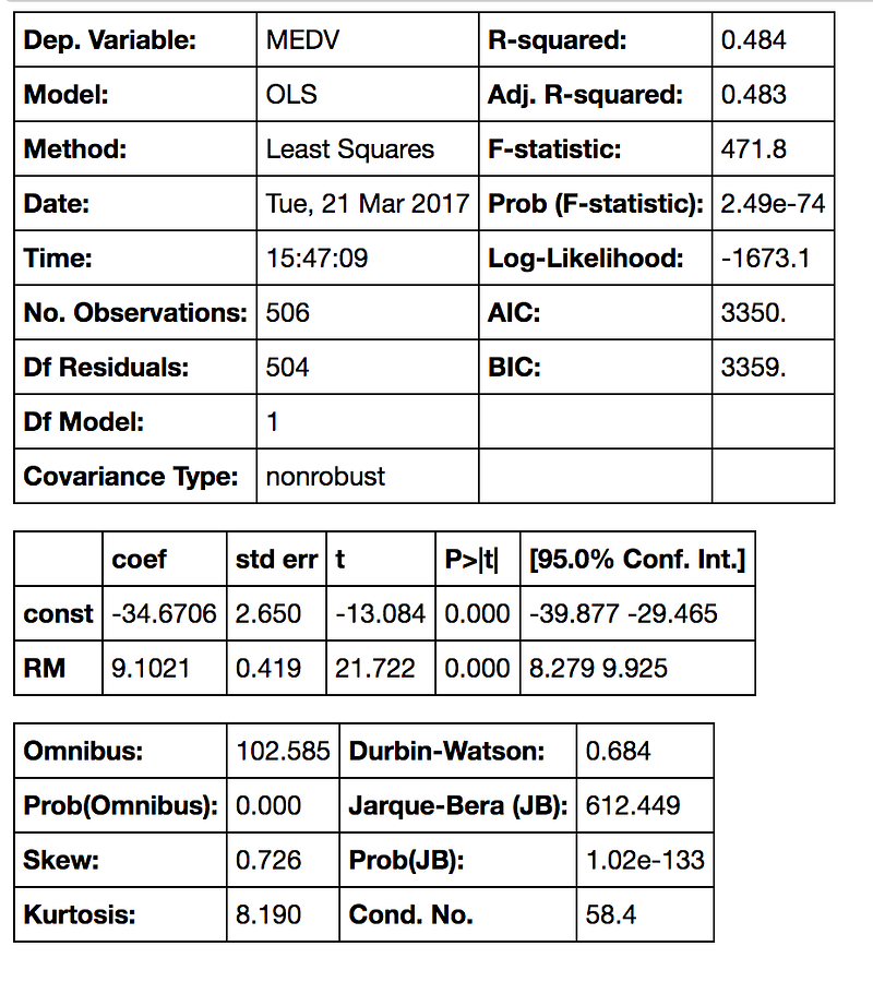
Interpreting the Table — With the constant term the coefficients are different. Without a constant we are forcing our model to go through the origin, but now we have a y-intercept at -34.67. We also changed the slope of the RM predictor from 3.634 to 9.1021.
Now let’s try fitting a regression model with more than one variable — we’ll be using RM and LSTAT I’ve mentioned before. Model fitting is the same:
X = df[[“RM”, “LSTAT”]]
y = target[“MEDV”]model = sm.OLS(y, X).fit()
predictions = model.predict(X)model.summary()And the output:
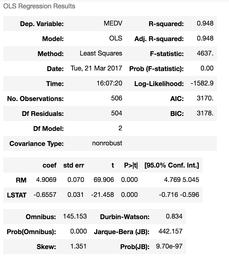
Interpreting the Output — We can see here that this model has a much higher R-squared value — 0.948, meaning that this model explains 94.8% of the variance in our dependent variable. Whenever we add variables to a regression model, R² will be higher, but this is a pretty high R². We can see that both RM and LSTAT are statistically significant in predicting (or estimating) the median house value; not surprisingly , we see that as RM increases by 1, MEDV will increase by 4.9069 and when LSTAT increases by 1, MEDV will decrease by -0.6557. As you may remember, LSTAT is the percentage of lower status of the population, and unfortunately we can expect that it will lower the median value of houses. With this same logic, the more rooms in a house, usually the higher its value will be.
This was the example of both single and multiple linear regression in Statsmodels. We could have used as little or as many variables we wanted in our regression model(s) — up to all the 13! Next, I will demonstrate how to run linear regression models in SKLearn.
Linear Regression in SKLearn
SKLearn is pretty much the golden standard when it comes to machine learning in Python. It has many learning algorithms, for regression, classification, clustering and dimensionality reduction. Check out my post on the KNN algorithm for a map of the different algorithms and more links to SKLearn. In order to use linear regression, we need to import it:
from sklearn import linear_modelLet’s use the same dataset we used before, the Boston housing prices. The process would be the same in the beginning — importing the datasets from SKLearn and loading in the Boston dataset:
from sklearn import datasets ## imports datasets from scikit-learn
data = datasets.load_boston() ## loads Boston dataset from datasets libraryNext, we’ll load the data to Pandas (same as before):
# define the data/predictors as the pre-set feature names
df = pd.DataFrame(data.data, columns=data.feature_names)

# Put the target (housing value -- MEDV) in another DataFrame
target = pd.DataFrame(data.target, columns=["MEDV"])So now, as before, we have the data frame that contains the independent variables (marked as “df”) and the data frame with the dependent variable (marked as “target”). Let’s fit a regression model using SKLearn. First we’ll define our X and y — this time I’ll use all the variables in the data frame to predict the housing price:
X = df
y = target[“MEDV”]
And then I’ll fit a model:
lm = linear_model.LinearRegression()
model = lm.fit(X,y)
The lm.fit() function fits a linear model. We want to use the model to make predictions (that’s what we’re here for!), so we’ll use lm.predict():
predictions = lm.predict(X)
print(predictions)[0:5]
The print function would print the first 5 predictions for y (I didn’t print the entire list to “save room”. Removing [0:5] would print the entire list):
[ 30.00821269 25.0298606 30.5702317 28.60814055 27.94288232]Remember, lm.predict() predicts the y (dependent variable) using the linear model we fitted. You must have noticed that when we run a linear regression with SKLearn, we don’t get a pretty table (okay, it’s not that pretty… but it’s pretty useful) like in Statsmodels. What we can do is use built-in functions to return the score, the coefficients and the estimated intercepts. Let’s see how it works:
lm.score(X,y)Would give this output:
0.7406077428649428This is the R² score of our model. As you probably remember, this the percentage of explained variance of the predictions. If you’re interested, read more here. Next, let’s check out the coefficients for the predictors:
lm.coef_will give this output:
array([ -1.07170557e-01,   4.63952195e-02,   2.08602395e-02,
         2.68856140e+00,  -1.77957587e+01,   3.80475246e+00,
         7.51061703e-04,  -1.47575880e+00,   3.05655038e-01,
        -1.23293463e-02,  -9.53463555e-01,   9.39251272e-03,
        -5.25466633e-01])
and the intercept:
lm.intercept_that will give this output:
36.491103280363134These are all (estimated/predicted) parts of the multiple regression equation I’ve mentioned earlier. Check out the documentation to read more about coef_ and intercept_.
So, this is has a been a quick (but rather long!) introduction on how to conduct linear regression in Python. In practice, you would not use the entire dataset, but you will split your data into a training data to train your model on, and a test data — to, you guessed it, test your model/predictions on. If you would like to read about it, please check out my next blog post. In the meanwhile, I hope you enjoyed this post and that I’ll “see” you on the next one.
Thank you for reading!


