Short Reads: SQL Window Functions with Engaging Examples

Introduction:

SQL window functions unlock the door to advanced data analysis by offering you the ability to create aggregated results without the need for grouping data or using nested queries. In this article, we will explore SQL window functions through captivating analogies, well-crafted examples, and visually engaging outputs that will help you understand and master these versatile functions.

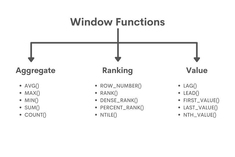
1. Overview of SQL Window Functions

Think of window functions as a kaleidoscope that enables you to isolate and manipulate specific data elements within your dataset while maintaining a connection to the whole picture. This powerful feature lets you perform calculations, aggregations, and rankings within a particular scope without changing the underlying data structure.

2. Practical Examples of Window Functions

Let’s dive into some practical examples that demonstrate window functions in action. We will provide queries, explanations of how they work, and the output for each function.

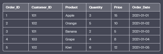
Example Dataset:

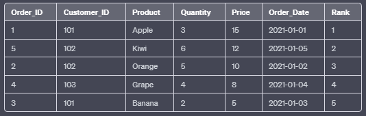
a. RANK():

The RANK() function assigns a unique rank to each row within the result set based on the specified column values. Rows with equal values receive the same rank, and the next rank is skipped.

SELECT Order_ID, Customer_ID, Product, Quantity, Price, Order_Date,
       RANK() OVER (ORDER BY Price DESC) AS Rank
FROM Orders;

In this example, the RANK() function orders the rows by the “Price” column in descending order. Rows with equal prices will receive the same rank.

Output:

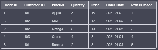
b. ROW_NUMBER():

The ROW_NUMBER() function assigns a unique number to each row within the result set based on the specified column values. Unlike RANK(), it does not skip any numbers even if rows have equal values.

SELECT Order_ID, Customer_ID, Product, Quantity, Price, Order_Date,
       ROW_NUMBER() OVER (ORDER BY Price DESC) AS Row_Number
FROM Orders;

In this example, the ROW_NUMBER() function orders the rows by the “Price” column in descending order. Each row will receive a unique number, regardless of whether their prices are equal.

Output:

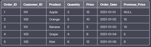
c. LAG():

The LAG() function returns the value from a previous row (or a specified number of rows before) in the result set. It is useful for comparing the current row’s value with a previous one.

SELECT Order_ID, Customer_ID, Product, Quantity, Price, Order_Date,
       LAG(Price) OVER (ORDER BY Order_Date) AS Previous_Price
FROM Orders;

In this example, the LAG() function retrieves the “Price” value from the previous row based on the “Order_Date” column.

Output:

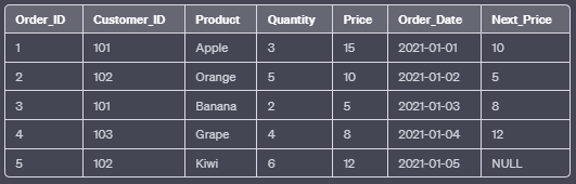
d. LEAD():

The LEAD() function returns the value from a subsequent row (or a specified number of rows after) in the result set. It is useful for comparing the current row’s value with the next one.

SELECT Order_ID, Customer_ID, Product, Quantity, Price, Order_Date,
       LEAD(Price) OVER (ORDER BY Order_Date) AS Next_Price
FROM Orders;

In this example, the LEAD() function retrieves the “Price” value from the next row based on the “Order_Date” column.

Output:

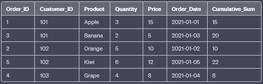
e. SUM():

The SUM() function calculates the sum of a set of values within a specified window frame.

SELECT Order_ID, Customer_ID, Product, Quantity, Price, Order_Date,
       SUM(Price) OVER (PARTITION BY Customer_ID ORDER BY Order_Date) AS Cumulative_Sum
FROM Orders;

In this example, the SUM() function calculates the cumulative sum of the “Price” column for each customer based on the “Order_Date” column.

Output:

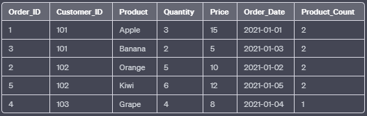
f. COUNT():

The COUNT() function counts the number of non-null values within a specified window frame.

SELECT Order_ID, Customer_ID, Product, Quantity, Price, Order_Date,
       COUNT(Product) OVER (PARTITION BY Customer_ID) AS Product_Count
FROM Orders;

In this example, the COUNT() function calculates the number of non-null “Product” values for each customer.

Output:

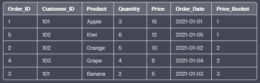
g. NTILE():

The NTILE() function divides the result set into a specified number of buckets and assigns a bucket number to each row. It is useful for breaking data into percentiles, quartiles, or other relative groupings.

SELECT Order_ID, Customer_ID, Product, Quantity, Price, Order_Date,
       NTILE(3) OVER (ORDER BY Price DESC) AS Price_Bucket
FROM Orders;

In this example, the NTILE() function divides the rows into three buckets based on the “Price” column in descending order.

Output:

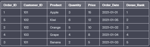
h. DENSE_RANK():

The DENSE_RANK() function assigns a unique rank to each row within the result set based on the specified column values. Unlike RANK(), it does not skip any rank numbers if rows have equal values.

SELECT Order_ID, Customer_ID, Product, Quantity, Price, Order_Date,
       DENSE_RANK() OVER (ORDER BY Price DESC) AS Dense_Rank
FROM Orders;

In this example, the DENSE_RANK() function orders the rows by the “Price” column in descending order. Rows with equal prices will receive the same rank, but no rank numbers are skipped.

Output:

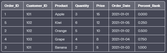
i. PERCENT_RANK():

The PERCENT_RANK() function calculates the relative rank of each row within the result set based on the specified column values. It returns a value between 0 and 1, with 0 being the lowest and 1 being the highest rank.

SELECT Order_ID, Customer_ID, Product, Quantity, Price, Order_Date,
       PERCENT_RANK() OVER (ORDER BY Price DESC) AS Percent_Rank
FROM Orders;

In this example, the PERCENT_RANK() function orders the rows by the “Price” column in descending order and calculates the relative rank as a percentage.

Output:

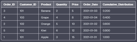
j. CUME_DIST():

The CUME_DIST() function calculates the cumulative distribution of each row within the result set based on the specified column values. It returns a value between 0 and 1, representing the proportion of rows with a value less than or equal to the current row’s value.

SELECT Order_ID, Customer_ID, Product, Quantity, Price, Order_Date,
       CUME_DIST() OVER (ORDER BY Price) AS Cumulative_Distribution
FROM Orders;

In this example, the CUME_DIST() function orders the rows by the “Price” column in ascending order and calculates the cumulative distribution.

Output:

Now that you’ve seen these captivating analogies, examples, and visual outputs for SQL window functions, you’ll be better equipped to apply them to your data analysis tasks. Mastering these functions will help you perform powerful calculations, aggregations, and rankings on your data, providing valuable insights for decision-making.

Thanks for Reading!

If you like my work and want to support me…

1. The BEST way to support me is by following me on Medium.
2. I share content about #dataengineering. Let’s connect on LinkedIn.
3. Feel free to give claps so I know how helpful this post was for you.